By: Johannes Korbmacher
Boolean algebra
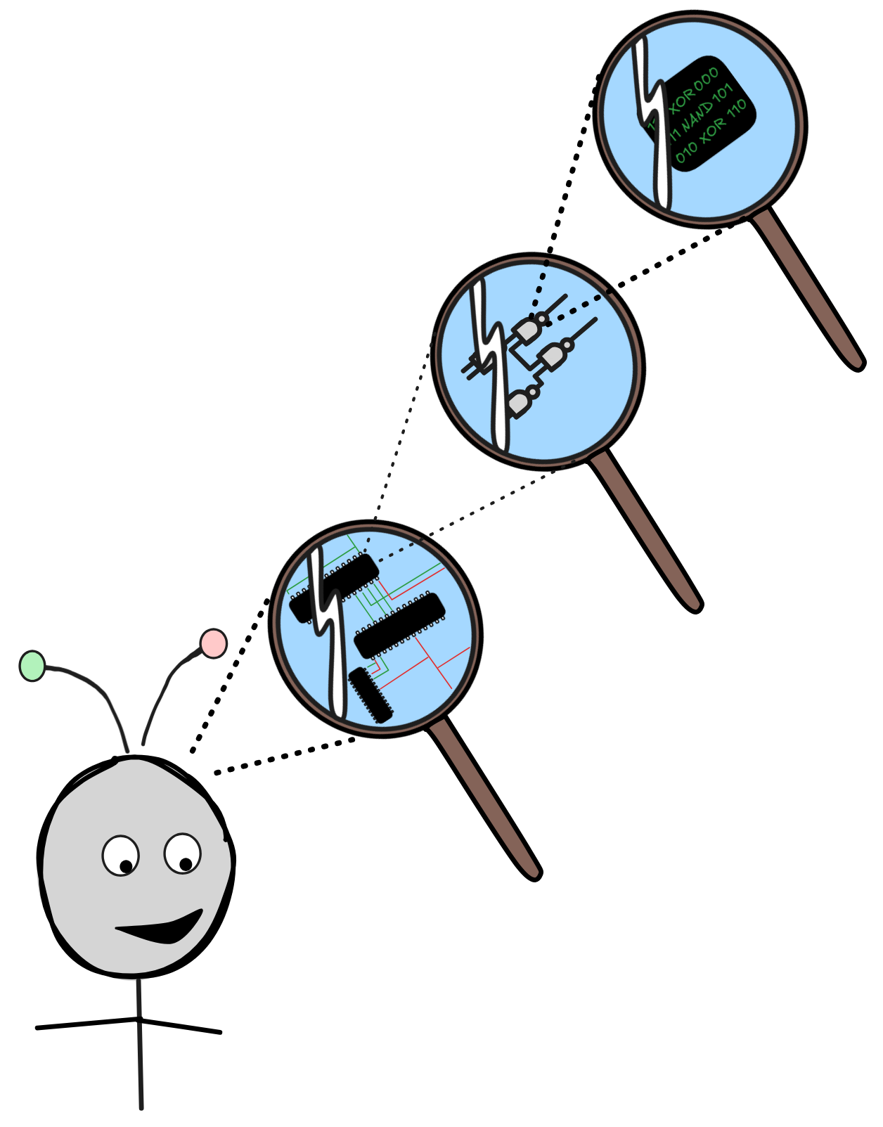 Boolean algebra—the logic of 0’s, 1’s, not, and, or, …—is the ultimate logical
foundation of modern computers, and by extension all AI systems. The study of
Boolean logic has its roots in the work of
George
Boole from the mid 19th century.
But it wasn’t until AI-pioneer
Claude
Shannon connected the theory to
the basic workings of electronic circuits that the importance of Boolean algebra
for the development of information technologies became apparent. While Shannon
was investigating
relays—essentially
electronically operated switches—and not
semiconductors, which are the
actual technology used to implement computers today, the fundamental principles
are the same. Boolean algebra is the logic of low-level computing, and the way
that computers add, subtract, multiply, etc. are ultimately grounded in Boolean
logic.
Boolean algebra—the logic of 0’s, 1’s, not, and, or, …—is the ultimate logical
foundation of modern computers, and by extension all AI systems. The study of
Boolean logic has its roots in the work of
George
Boole from the mid 19th century.
But it wasn’t until AI-pioneer
Claude
Shannon connected the theory to
the basic workings of electronic circuits that the importance of Boolean algebra
for the development of information technologies became apparent. While Shannon
was investigating
relays—essentially
electronically operated switches—and not
semiconductors, which are the
actual technology used to implement computers today, the fundamental principles
are the same. Boolean algebra is the logic of low-level computing, and the way
that computers add, subtract, multiply, etc. are ultimately grounded in Boolean
logic.
But the importance of Boolean algebra to AI is not restricted to the low level.
Propositional reasoning on all levels follows the laws of Boolean algebra.
Conditionals
in most programming languages, such as C, Python, or Java, rely on Boolean
connectives:
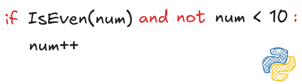 To write good conditionals and understand code that others have written, you
need a solid understanding of Boolean logic.
To write good conditionals and understand code that others have written, you
need a solid understanding of Boolean logic.
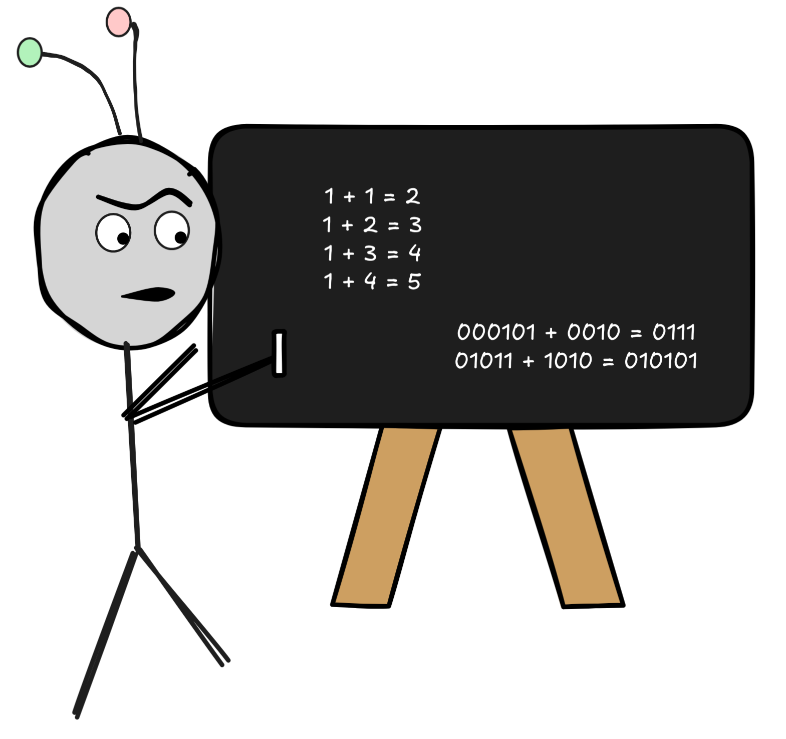
Even on the highest level, deductive reasoning with propositional information stored in KBs follows the laws of Boolean algebra:
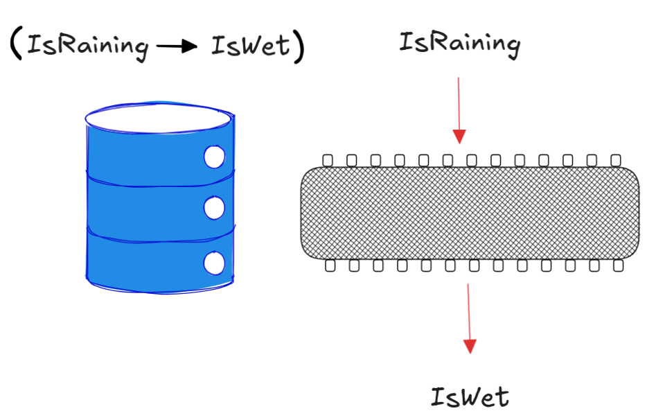
In short, the importance of Boolean logic for AI can hardly be overstated.
At the end of this chapter, you’ll be able to:
-
explain the basic principles of Boolean algebra
-
implement the Boolean truth-functions using simple circuits
-
derive logical laws from the Boolean laws
-
build and apply adders from Boolean circuits
-
test propositional inferences for deductive validity using Boolean models
Boolean truth-values
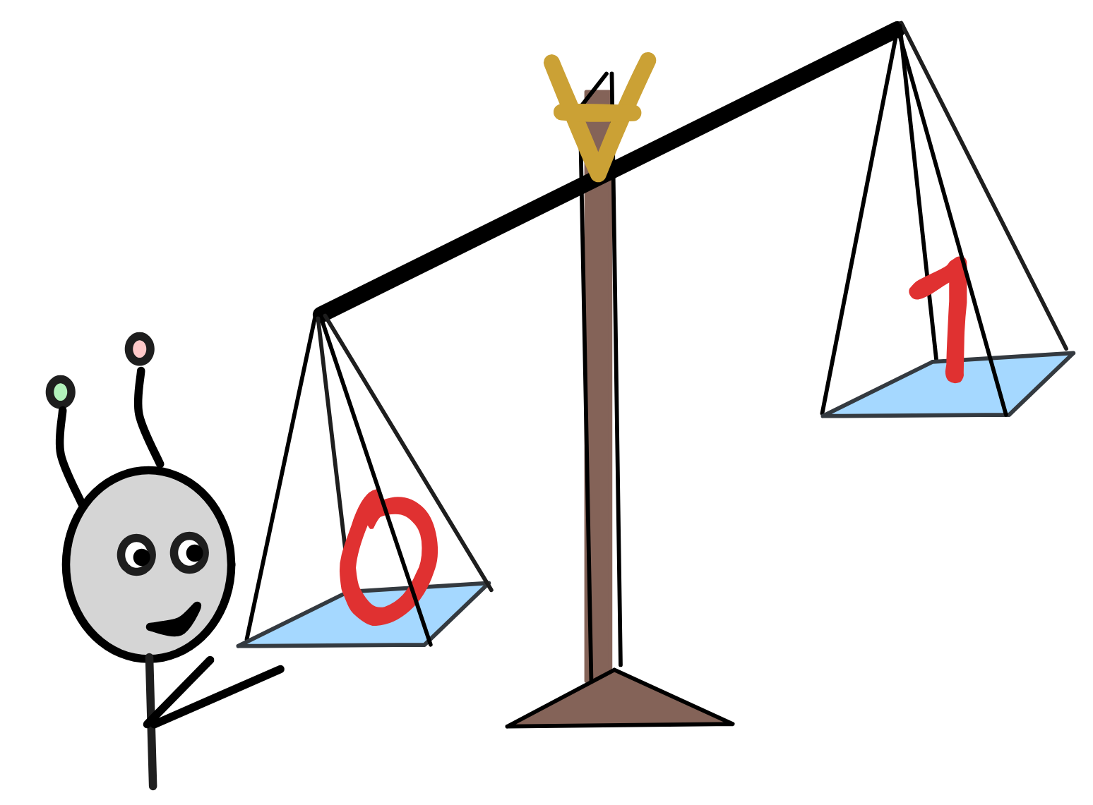
Boolean algebra is the logic of the proverbial 0’s and 1’s. That is, the Boolean truth-values are:
These values have many different interpretations depending on the reasoning context we’re in: on/off, high/low, true/false, ….
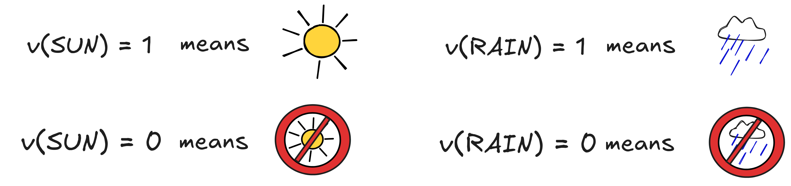
In logic, the true/false interpretation is the most common. If we’re dealing with a propositional language that has a propositional letter SUN to express that the sun is shining, assigning it the value 1 means that the sun is indeed shining, while assigning SUN the value 0 means that it is not.

In Boolean logic, there is no third truth-value for facts that are undecided, unknown, indeterminate. From a logical perspective, this is a modelling assumption, which means that Boolean logic is only applicable in situations, where things are clear-cut, true or false. But luckily, there are many such situations, ranging from the behavior of semiconductors to simple facts of everyday life.
Truth-functions
The basic operations of Boolean algebra are the so-called truth-functions. These are functions in the mathematical sense, which take one or more Boolean truth-values as input and return exactly one Boolean truth-value as output.
For now, we’ll restrict ourselves to the basic functions NOT, AND, and OR. These are not the most fundamental truth-functions in any sense of the word, but are the most commonly used truth-functions in logical theory. In computer science, instead, especially when we’re thinking about basic semiconductor circuits XOR and especially when we’re thinking about basic semiconductor circuits NAND are more commonly used as basic functions.
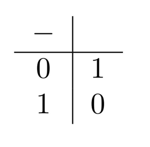
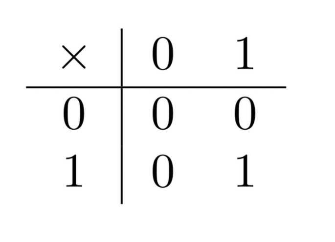
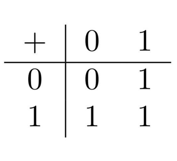
The truth-functions are given by the following functional tables, where the first input is in the first column and the second input in the first row. In the case of the binary functions—the ones with two inputs—the output is read-off by intersecting the two input columns:
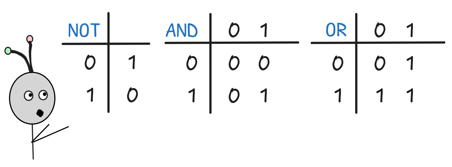
So, for example, NOT 0 = 1 and 1 OR 0 = 1.
The truth-functions NOT, AND, and OR are sufficient to express any truth-function whatsoever. This mathematical fact is known as the joint truth-functional completeness of these operators, and we’ll investigate it in the exercises. NOT, AND, and OR are not the only collection of truth-functions with this property, not even the smallest one. But especially in logical contexts, they are the most commonly used ones, since using these truth-functions, we can easily describe many different important concepts and algorithms with relative ease.
To get a better understanding of how these truth-functions work, we’ll look at an implementation using relays—essentially tracing some of Shannon’s ideas. A relay is, essentially, an electronically operated switch. For our purposes, we’ll work with the following two kinds of relays:
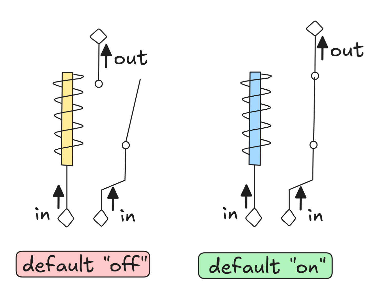
Both relays have two inputs and one output. One input leads to an electromagnet, which if it receives power exerts a magnetic force on the switch connected to the other input and flips it. In the default "off" relay, this closes the circuit and the output receives power in case the input does. With the default "on" relay, it’s the other way around: if the electromagnet receives power, the output gets disconnected from the input, breaking the circuit.
So, if the default “on” circuit receives constant power to the right circuit, this is how turning the power to the magnet off and on affects the behavior of the circuit:
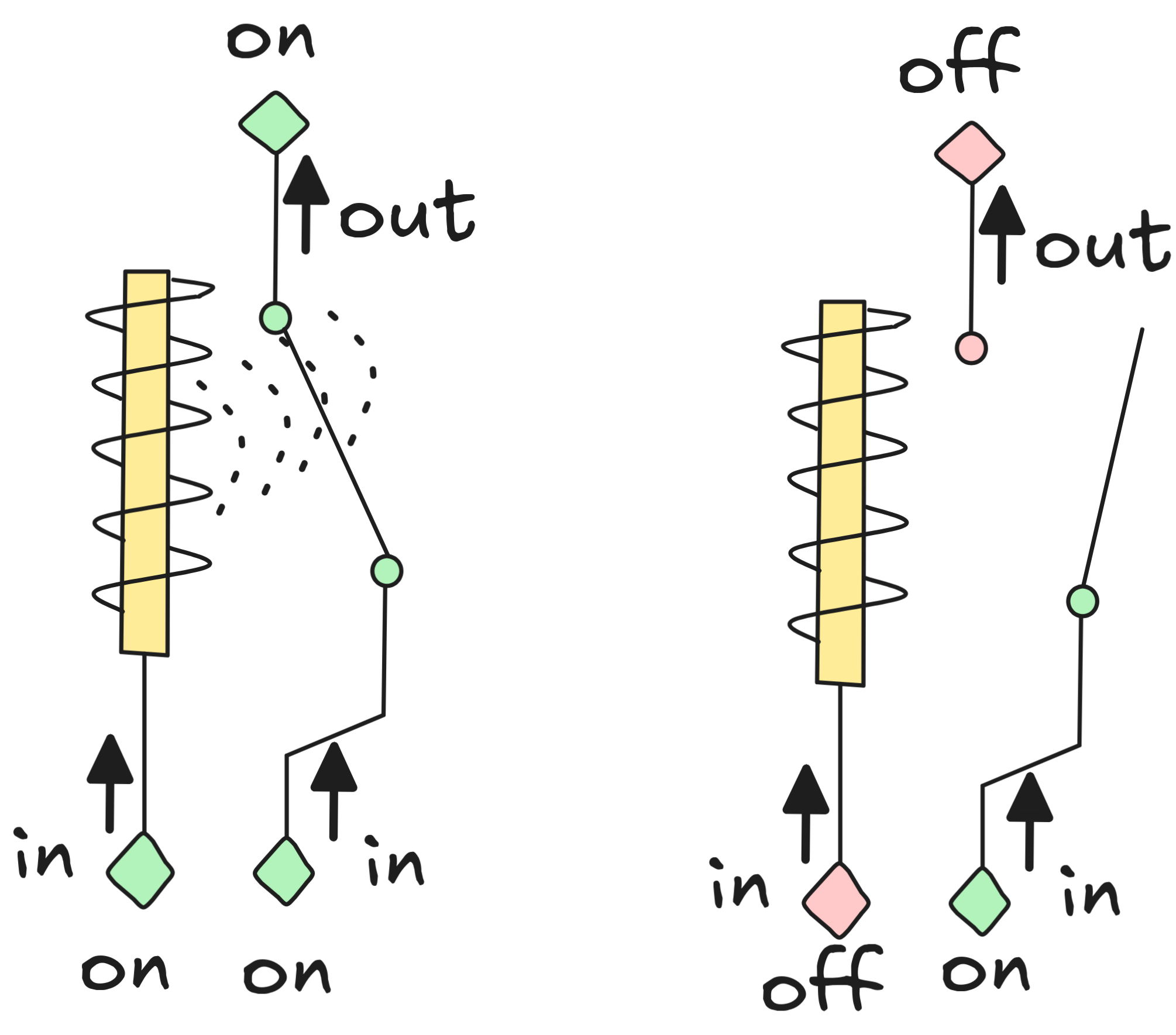
The default “on” relay, of course, behaves dually.
We can use these two relays to implement our three Boolean truth-functions. For this, we assume that following set-up:
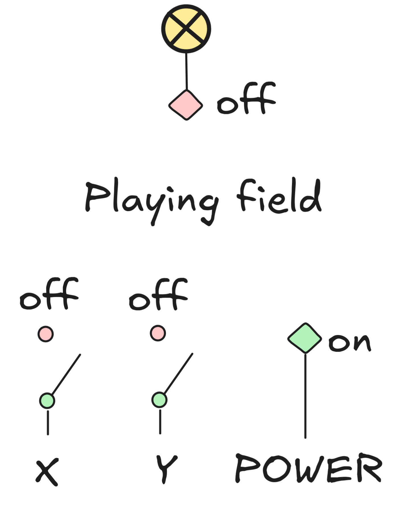
We have:
-
a constant source of power POWER
-
two switchable inputs, X and Y
-
a single output, which is connected to an indicator lamp
We interpret X being off as the first input being 0 and X being on as the first input being 1, and analogously for Y and the second input. The lamp represents the output in the same way: if it is off, the output is 0, if it is on the output is 1. So, the set-up is depicted in the configuration for the first and second input both being 0. Since we haven’t implemented anything yet, the output is also 0.
We can implement the NOT function with a single default “on” relay:
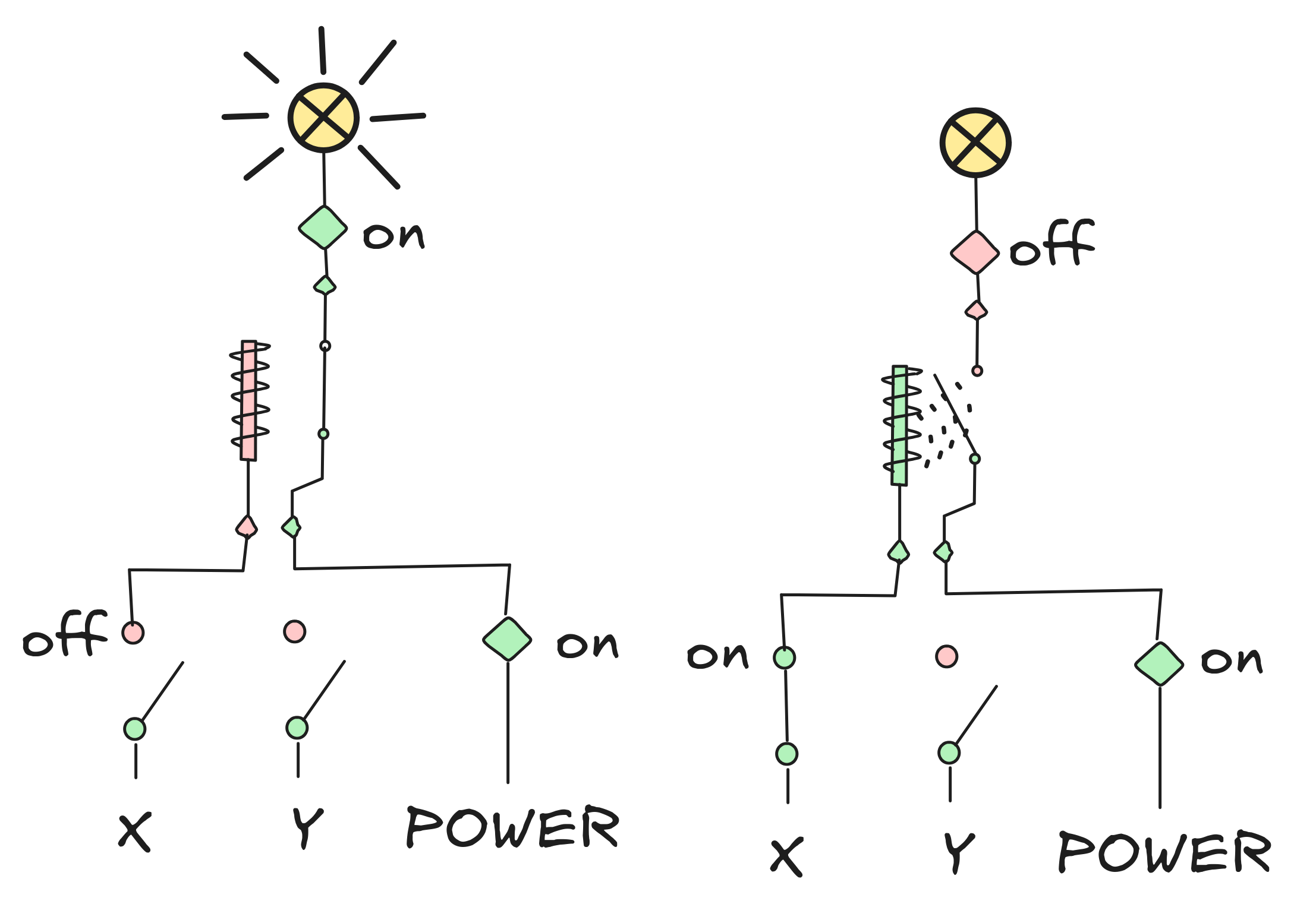
Depicted are both states of the circuit: if the first input is 0 (X is off), the output is 1 (the lamp is on); and if the first input is 1 (X is on), the output is 0 (the lamp is off). The second input doesn’t matter, of course.
We can implement AND using the other kind of relay as follows:
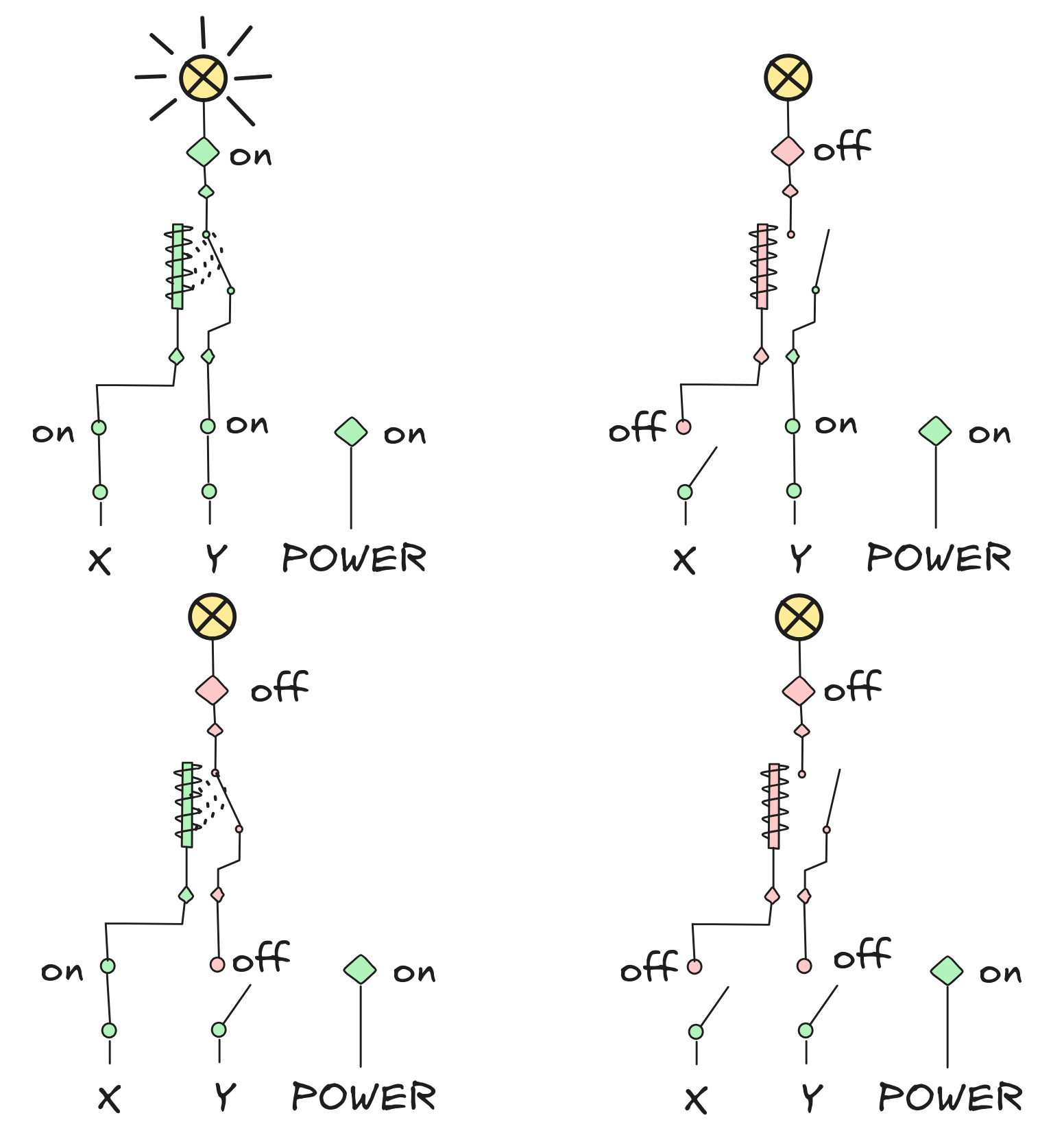
There are four possible states of the circuits, but as you can see: only if both inputs are 1 the output is 1. In all other configurations, the output is 0—just like the AND function, requires.
Implementing the OR function using the relays is one of the exercises. If you want to try more, you can try the amazing nandgame, which allows you to implement an entire computer “by hand”.
The Laws of Boolean algebra
 The behavior of the Boolean truth-functions is
governed by a series of algebraic laws, that is identities describing
their interaction. These identities are formulated using variables X,Y,…,
which can assume arbitrary values from among the set {0, 1}. Take, for
example, the Boolean equation:
The behavior of the Boolean truth-functions is
governed by a series of algebraic laws, that is identities describing
their interaction. These identities are formulated using variables X,Y,…,
which can assume arbitrary values from among the set {0, 1}. Take, for
example, the Boolean equation:
(X AND Y) = (Y AND X)
This equation says that for any pair of values X,Y from {0, 1} , the result of applying AND with X as the first input and Y as the second is the same as applying AND with Y as the first input and X as the second.
You can verify this law by inspecting the function table for AND and going through all possible values for X and Y. Here are the corresponding calculations:
(0 AND 0) = (0 AND 0)
(0 AND 1) = 0 = (1 AND 0)
(1 AND 0) = 0 = (0 AND 1)
(1 AND 1) = (1 AND 1)
Only the second and third line are “interesting” calculations, the first and last are “trivial”.
This law is called the law of Commutativity for AND, which states that for AND, the order of its inputs doesn’t matter. Many laws of Boolean algebra have such names.
Here are the most important laws and their corresponding names:
(X OR (Y OR Z)) = ((X OR Y) OR Z)(X AND (Y AND Z)) = ((X AND Y) AND Z) |
(“Associativity”) | |
(X OR Y) = (Y OR X)(X AND Y) = (Y AND X) |
(“Commutativity”) | |
(X OR (X AND Y) = X (X AND (X OR Y) = X |
(“Absorption”) | |
(X OR (Y AND Z)) = ((X OR Y) AND (X OR Z) (X AND (Y OR Z)) = ((X AND Y) OR (X AND Z) |
(“Distributivity”) | |
(X OR NOT X) = 1 (X AND NOT X) = 0 |
(“Complementation”) | |
(X OR 0) = X (X AND 1) = X |
(“Identity”) | |
(X AND 0) = 0 (X OR 1) = 1 |
(“Domination”) | |
You can (and should!) verify all these laws, just like we did for Commutativity. Don’t worry, you don’t need to memorize all of these laws. But at the same time, knowing them can be incredibly helpful in showing facts about Boolean algebras.
In particular, you can use these laws to derive other laws in an algebraic way, that is by manipulating equations. For example, you can derive the following important family of laws known as the de Morgan laws:
NOT (X OR Y) = (NOT X AND NOT Y)NOT (X AND Y) = (NOT X OR NOT Y) |
(“De Morgan Identities”) | |
NOT NOT X = X |
(“Double Negation”) | |
Let’s look at how to derive ("Double Negation") :
-
We start with
NOT NOT X = ((NOT NOT X) AND 1),which we know by “Identity”.
-
We then apply the fact that
X OR NOT X = 1, that is “Complementation”, which gives us thatNOT NOT X = ((NOT NOT X) AND (X OR NOT X)), -
By “Distributivity”, we have
((NOT NOT X) AND (X OR NOT X))= ((NOT NOT X) AND X) OR ((NOT NOT X) AND NOT X),so we can conclude that
NOT NOT X = ((NOT NOT X) AND X) OR ((NOT NOT X) AND NOT X). -
Now, notice that
((NOT NOT X) AND NOT X) = 0by “Complementation”. So step 3. simplifies to:NOT NOT X = ((NOT NOT X) AND X) OR 0.which by “Identity” simplifies further down to:
NOT NOT X = (NOT NOT X) AND X. -
Going a bit faster, we can see by analogous reasoning that
X = X AND 1 = X AND ((NOT NOT X) OR NOT X),using “Identity” and “Complementation” like before.
-
Using “Distributivity”, this gives us
X = (X AND NOT NOT X) OR (X AND NOT X). -
But since
(X AND NOT X) = 0, we now getX = (X AND (NOT NOT X))using “Identity” and “Complementation”.
-
But now we know that both:
NOT NOT X = (NOT NOT X) AND XX = (X AND (NOT NOT X)),
where the latter is just X = (NOT NOT X) AND
X, using “Commutativity” to reorder. So, we can conclude that:
NOT NOT X = X
This derivation may seem a bit tedious—especially since we can prove the fact
that NOT NOT X = X fact by simply inspecting
the function tables: NOT NOT 1 = 1 and NOT NOT 0 = 0.
But there are also questions where the laws are much more efficient at giving you the answer than inspecting the tables. Take for example the Boolean expression:
  X AND ((Y
  AND Z) OR NOT (Y
  AND Z))
It turns out that this expression reduces to simply X. To see this by truth-table inspection, we need to go through 2³ = 8 different combinations of truth-values for X, Y, Z and for each combination, we need to calculate 5 different operations. That’s a lot of calculations.
Using the laws of Boolean algebra, however, we can recognize that
((Y AND Z) OR NOT (Y AND Z))
is of the form
[something] OR NOT [something],
where [something] = (Y AND Z). So, by
“Complementation”, we can reduce
X AND ((Y
AND Z) OR NOT (Y
AND Z))
X AND 1,
which by “Identity” is just X.
 The derivation also illustrates an important point: the above laws of Boolean
algebra allow us to derive further laws that don’t look like they’re covered by
the initial list. In fact, we can derive all valid identities of Boolean
algebra from these laws. The list of laws is complete in this sense.
Having a complete list of laws for a subject matter is an incredibly feat: all
there is to know about Boolean algebras is encoded in these laws. And as the
example of
The derivation also illustrates an important point: the above laws of Boolean
algebra allow us to derive further laws that don’t look like they’re covered by
the initial list. In fact, we can derive all valid identities of Boolean
algebra from these laws. The list of laws is complete in this sense.
Having a complete list of laws for a subject matter is an incredibly feat: all
there is to know about Boolean algebras is encoded in these laws. And as the
example of X AND ((Y AND Z) OR NOT (Y AND Z)) shows, this
can be a handy tool in the toolbox of any AI researcher.
On a more historical note, the set of laws we’ve discussed are originally due to Alfred North Whitehead. But it is not the only collection of complete laws and certainly not the minimal one. It turns out that the following single law is enough to derive all the other laws of Boolean algebra (expressed using only NOT and OR):
NOT (NOT (NOT (X OR Y) OR Z) OR NOT (X OR NOT (NOT Z OR NOT (Z OR U)))) = Z
But that’s a story for another day.
Adders
To illustrate the usefulness of Boolean algebra, let’s look an important application: the implementation of addition via adders.
 An adder is a circuit that performs addition on numbers. We can implement
adders using Boolean truth-functions, but first, we need to translate the
numbers into something a Boolean function can understand. We need to talk about
binary numbers.
An adder is a circuit that performs addition on numbers. We can implement
adders using Boolean truth-functions, but first, we need to translate the
numbers into something a Boolean function can understand. We need to talk about
binary numbers.
The fundamental idea of binary numbers is that we can represent any natural number as a sequence of 0’s and 1’s. Here’s how this works. Take the string
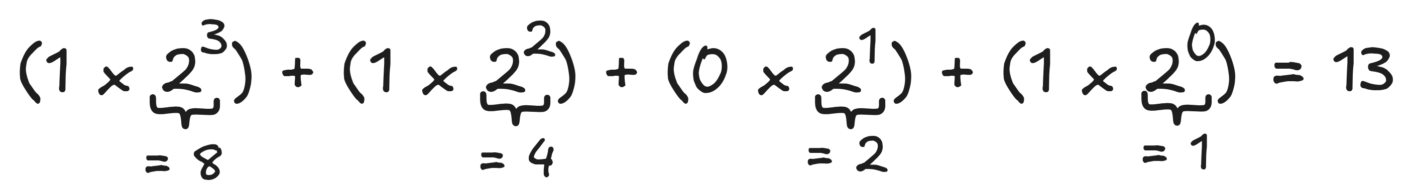
The 0’s and 1’s are also called bits—short for binary digits—especially in computer science contexts. For simplicity, we count the bits of a binary number backwards from the end of the string (right-to-left rather than left-to-right). You’ll see in a second why. We also start counting at 0, which might be unusual at first, but is also common in computer science. So, the first bit of 1101, for example, is what would normally be called “the second digit from the end”, i.e. 0:
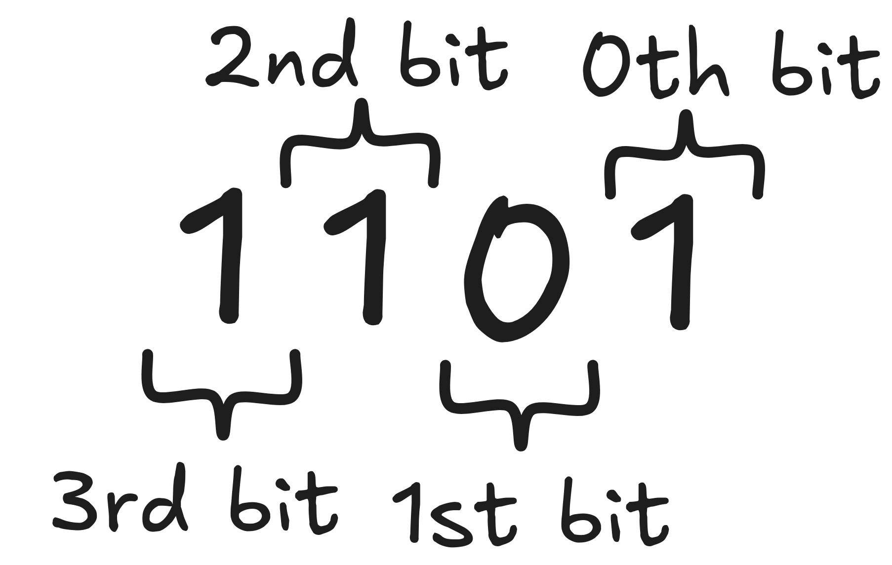
To calculate the number represented by a string, you go through the digits one. Let’s call the nth bit dₙ. So, in our example, we have:
Then you multiply the n-th bit with the n-th power of 2, that is, you calculate:
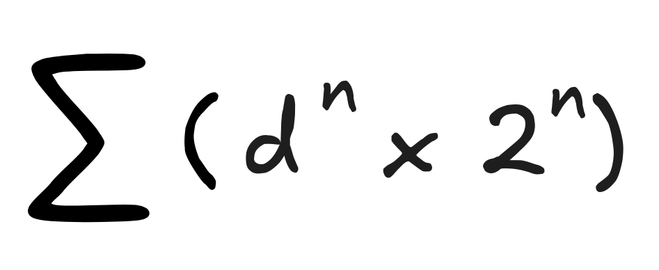
But this is just “fancy notation”" to say exactly the same thing we just said.
The number 1101 is what’s called a 4-bit number, since it represents a number using four bits. Typically, we’re dealing with binary numbers of a fixed number of bits. In implementations, this restriction is enforced by hardware limitations: while mathematicians are happy dealing with strings of infinite length in their minds, it’s slightly complicated to stuff them into a computer chip. This is why we have 64-bit computing and not “∞-bit computing”.
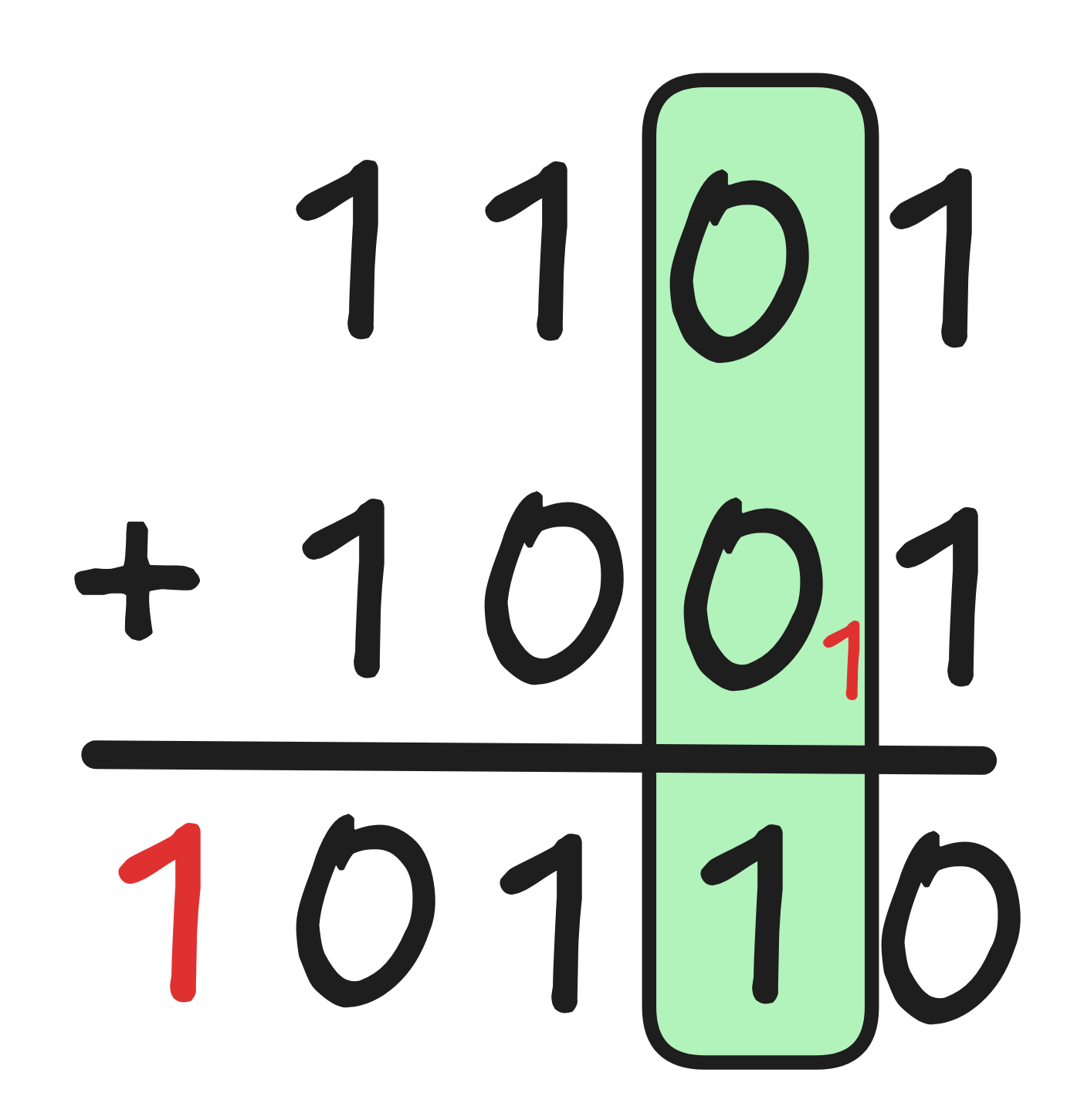
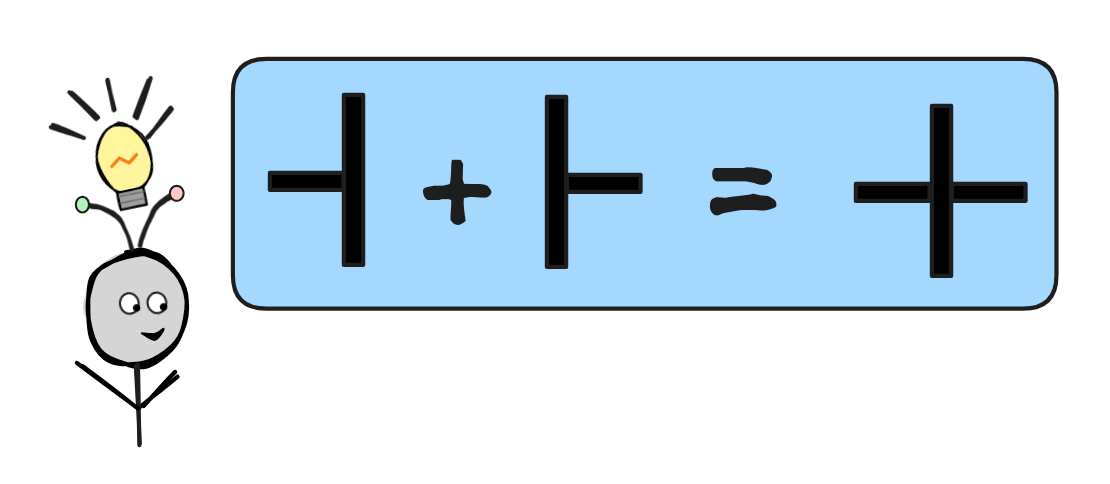
But there are also practical advantages to have a fixed bit-size. For example, if we have two binary numbers of the same length, they are incredibly easy to add. Here’s an example of how this works:
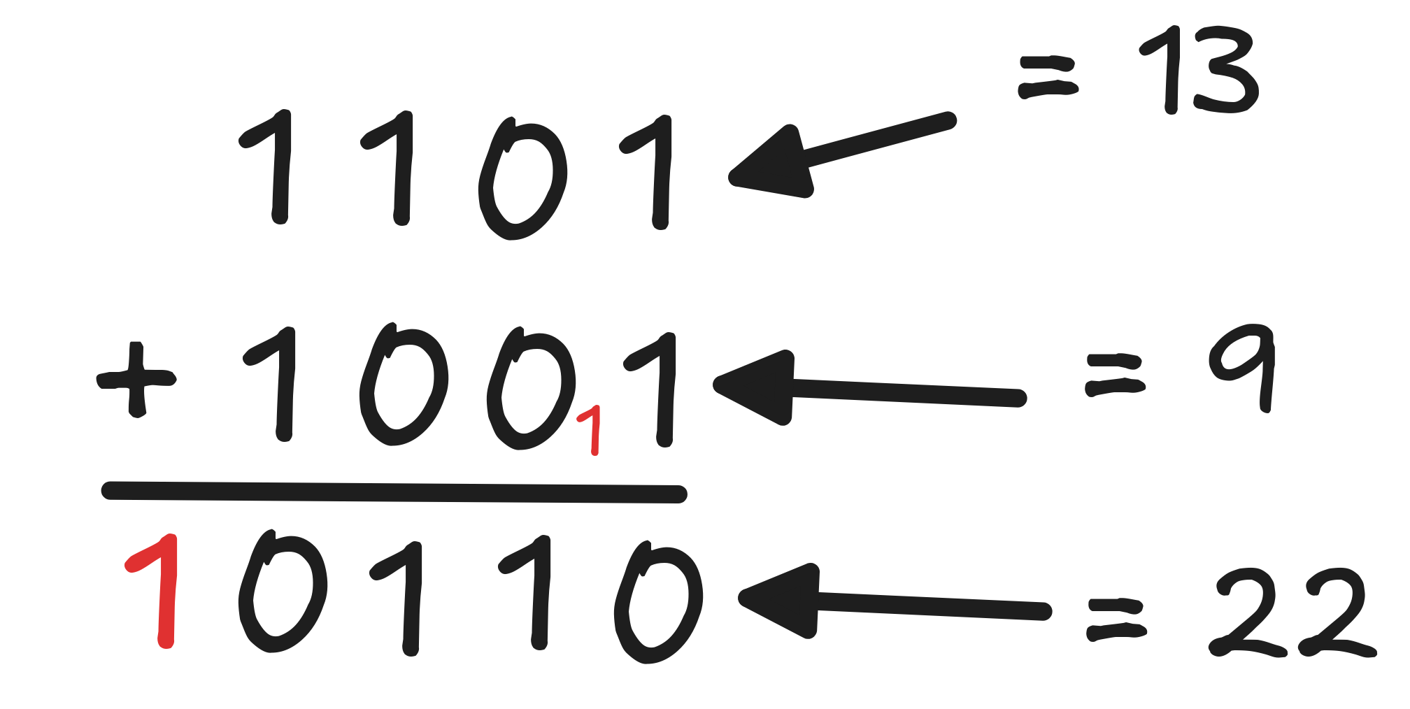
Essentially, what we do here is to add the two numbers by adding their binary components one by one, taking care along the way to “carry over” any overspill. The way this works is that you start from the end again and you add the two 0th digits according to the following rules:
-
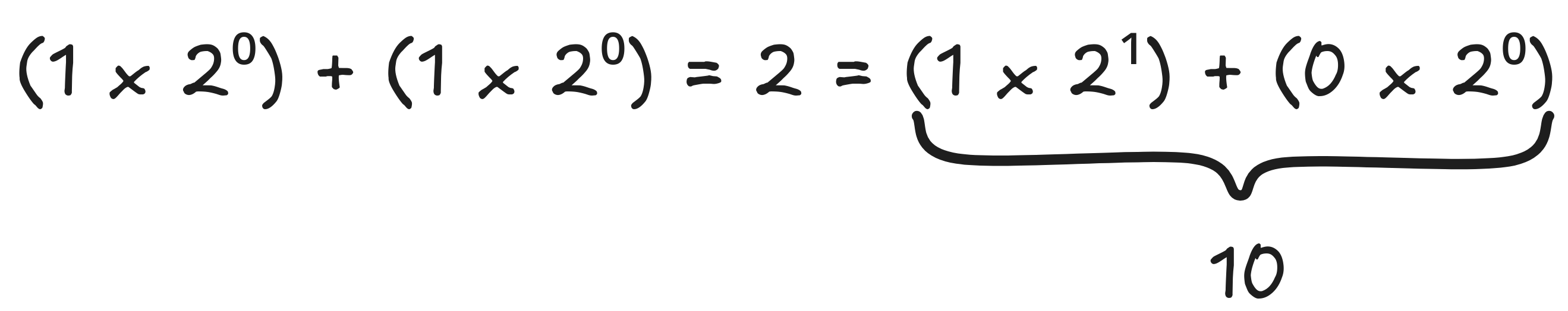
If one digit is a 0 and the other is a 1, the result is 1, since
(0 x 2⁰) + (1 x 2⁰) = (1 x 2⁰) + (0 x 2⁰) = 1 -
If both digits are a 0, then the result is 0, since
-
If both digits are a 1, then the result is 0 with a carry of 1 (this is the little red number in the next column), since
Now you might already see that what’s going on here is just Boolean truth-functions being applied to the 0th digit. Basically, what we have here are two inputs: the 0th digit of our first number and the 0th digit of our second number. Let’s call them d₀ and e₀ respectively. What we need to calculate are two things: the 0th digit of our result, and any potential carry.
According to the rules, the first output, the 0th digit of our addition, is 1 just in case exactly one (and not both) of d₀ and e₀ is 1. Otherwise, if either d₀ = e₀ = 0 or d₀ = e₀ = 1, the output is 0. This describes a truth-function, which is known as XOR (“exclusive or”), which has the following function table:
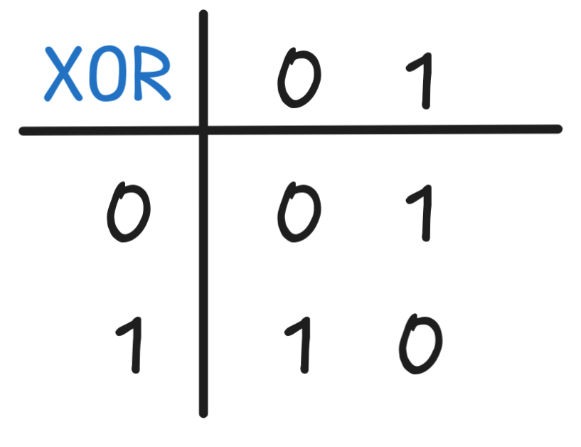
We can actually express this function using only NOT, AND, OR, but using XOR directly it’s much easier.
The carry, instead, is 1 just in case both d₀ and e₀ are 1 and 0 otherwise. But that’s just the specification of AND. So, we can describe the rule as follows using Boolean truth-functions:
-
the 0th digit of our addition is d₀ XOR e₀
-
the carry is d₀ AND e₀
If we’ve implemented XOR and AND using relays or semiconductors, following the ideas sketched above, we can implement this rule using the following circuit known as a half-adder:
 The idea is that the blue boxes are implementations of XOR and AND
respectively, which take two inputs and give two outputs. The input switches
represent d₀ and e₀ respectively, on meaning 1 and off meaning 0. The
two lamps stand for the results, the 0th digit and the carry, respectively. A
lamp being on means the relevant output is 1, otherwise its 0. What’s
depicted here is the configuration that corresponds to our example, i.e. d₀ =
1 and e₀ = 1.
The idea is that the blue boxes are implementations of XOR and AND
respectively, which take two inputs and give two outputs. The input switches
represent d₀ and e₀ respectively, on meaning 1 and off meaning 0. The
two lamps stand for the results, the 0th digit and the carry, respectively. A
lamp being on means the relevant output is 1, otherwise its 0. What’s
depicted here is the configuration that corresponds to our example, i.e. d₀ =
1 and e₀ = 1.
Now, let’s return to the 1st (meaning second from the end) digit of our result:
You might notice that here, we no longer have just two inputs, but three: the 1st digit of the first summand (d₁), the 1st digit of the second summand (e₀), plus the carry from the previous step (let’s call it c₀). Like in the first step, we need to calculate two outputs: the 1st digit of our sum, and any potential carry that might result.
The 1st digit of our sum is rather straight-forward to calculate: it should be 1 just in case exactly one input is 1 or all three inputs are 1. The reasoning is like in the two input case from before:
-
If there’s no 1, we get:
(0 x 2¹) + (0 x 2¹) + (0 x 2¹)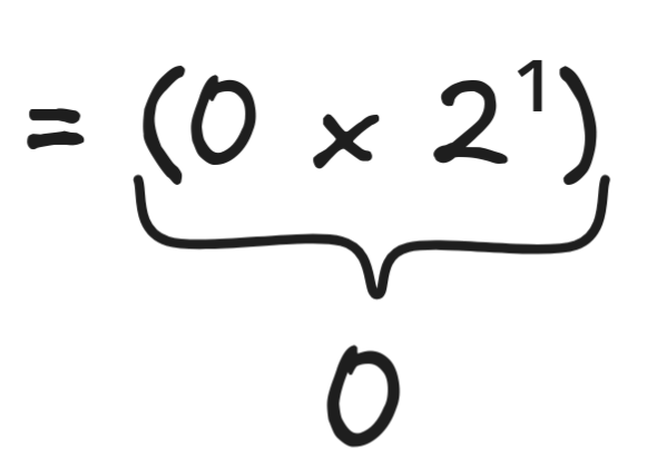
-
If there’s precisely one 1, we have:
(1 x 2¹) + (0 x 2¹) + (0 x 2¹)= (0 x 2¹) + (1 x 2¹) + (0 x 2¹)= (0 x 2¹) + (0 x 2¹) + (1 x 2¹)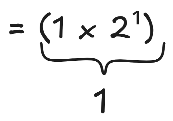
-
If there’s exactly two 1’s, we get:
(1 x 2¹) + (1 x 2¹) + (0 x 2¹)= (1 x 2¹) + (0 x 2¹) + (1 x 2¹)= (0 x 2¹) + (1 x 2¹) + (1 x 2¹)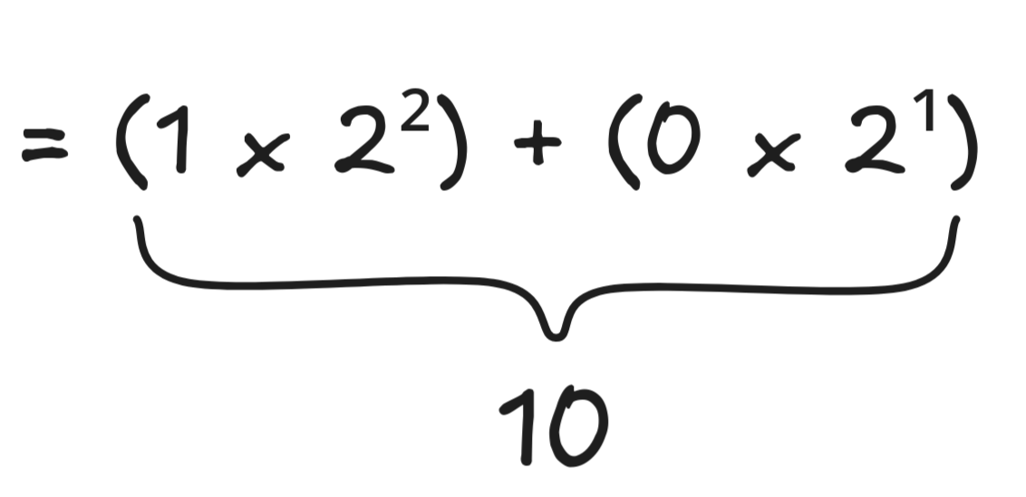
-
And if there’s three 1’s, we have:
= (1 x 2¹) + (1 x 2¹) + (1 x 2¹)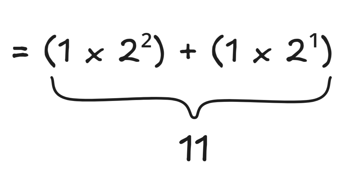
The Boolean truth-function which gives us precisely the desired output for the 1st digit of our computation is:
But what should the carry be? Inspecting the cases, we can see that we should carry a 1 in one of two scenarios: if there’s exactly two 1’s and if there’s precisely three. How can we express this in terms of truth-functions? While there are different ways of doing this, here’s a common one using AND, OR, and XOR:
The reasoning is that we can analyze our two scenarios (exactly two 1’s and exactly three 1’s) in a slightly different way: either both inputs are 1 or exactly one input is 1 and the carry from before is 1. You can—and— should!—verify that this works.
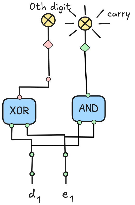
It’s a bit more tedious to implement this using circuits, but of course it can be done:
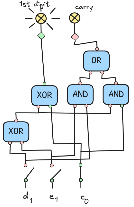
This circuit, here depicted in the configuration from our example, is called a
full adder, and can also be implemented using two half adders.
We can use full adders to implement full addition on fixed-bit integers: just chain full adders to calculate the individual output bits, ensuring to always carry over when necessary.
This example shows that Boolean inference is at the very heart of computation and its implementation: one of the—if not the—most basic mathematical operations is implemented using Boolean logic. In fact, addition becomes a form of Boolean inference.
Models
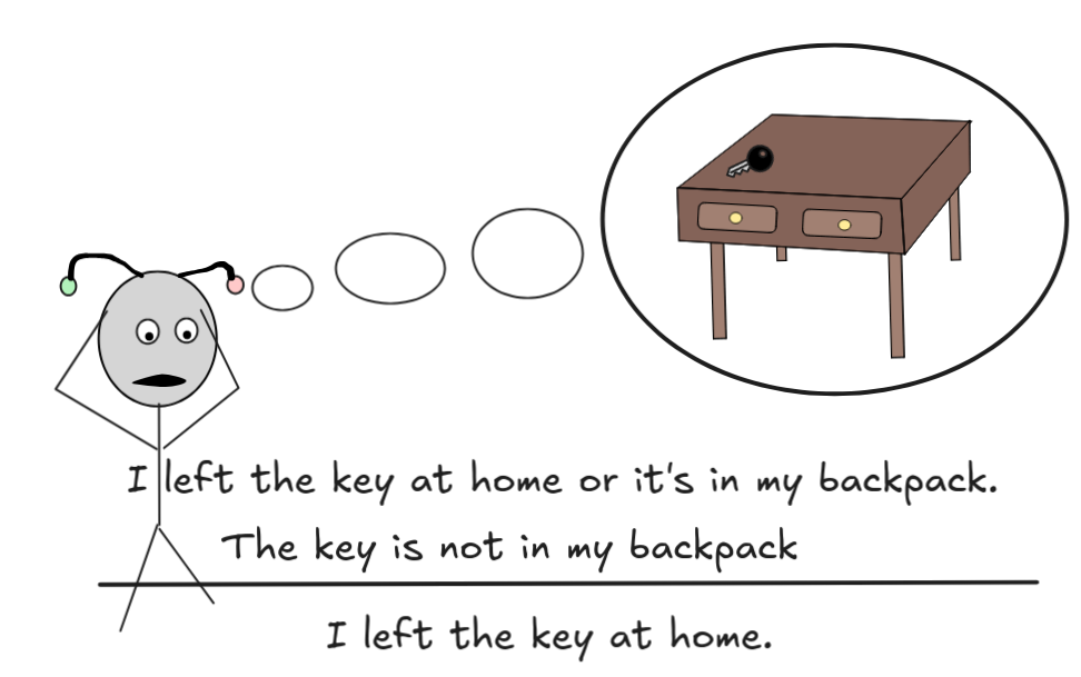
Turning from low-level reasoning—viz. the implementation of arithmetic—to more high-level reasoning, we look at deductive reasoning in propositional logic next. This is the kind of inference that is involved in conditionals in programming languages, but also in automated inference with KB’s, for example in expert systems. It is common in everyday reasoning, as well, when we make inferences like:
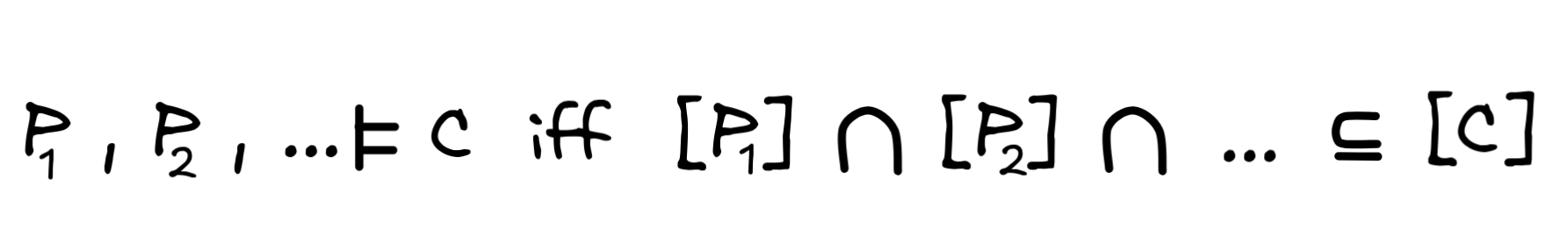
We can use Boolean algebra to define the notion of a model for a propositional language. This will give us the notion of deductively valid inference using the schema:
In essence what we need to do is very similar to the case of addition above: before we could implement addition using Boolean algebra, we needed to translate numbers into something that Boolean algebra can understand. Essentially, we need to do the same thing for logic: before we can apply Boolean algebra to inferences, we need to translate the formulas of our formal language into something that Boolean algebra can work with—which turns out to be truth-values.
Suppose that we have a propositional language, L, which has two propositional variables SUN and RAIN, which we interpret as saying that it’s sunny and that it’s rainy, respectively.
There are four logically relevant reasoning scenarios for inference in this language. It could be:
-
Sunny and rainy.
-
Sunny, but not rainy.
-
Not sunny, but rainy.
-
Neither sunny, nor rainy.
That is, our logical space should look something like this:

Our aim is to implement a definition of a model for L that adequately reflects this idea. To achieve this goal, we’ll use the thought mentioned before that we can assign truth-values to propositional variables, where assigning the value 1 to SUN, say, means that SUN is true (it’s sunny), and assigning it the value 0 means that SUN is not true (it’s not sunny).
Mathematically, we typically express such an assignment of values using the function symbol v, like so:
When more than one assignment viewed as a model is under consideration at the same time, we disambiguate with the use of subscripts. So, for example, there is the assignment v₁, such that v₁(SUN)=1 and v₁(RAIN)=1, as well as the assignment v₂, such that v₂(SUN)=1, but v₂(RAIN)=0.
Since there are two propositional variables (SUN and RAIN), there are 2² = 4 possible ways of assigning truth-values from among {0, 1} in this way. Each of these assignments corresponds to one of our reasoning situations. More generally, if there are n propositional variables, where n is any number, then there are 2ⁿ different ways of assigning truth-values from {0, 1} to the propositional variables. In our case, the relevant assignments and corresponding scenarios are:
M₁:

|
v₁(RAIN) = 1 and v₁(SUN) = 1 | M₃:

|
v₃(RAIN) = 0 and v₃(SUN) = 1 | |||
M₂:

|
v₂(RAIN) = 1 and v₂(SUN) = 0 | M₄:

|
v₄(RAIN) = 1 and v₄(SUN) = 1 | |||
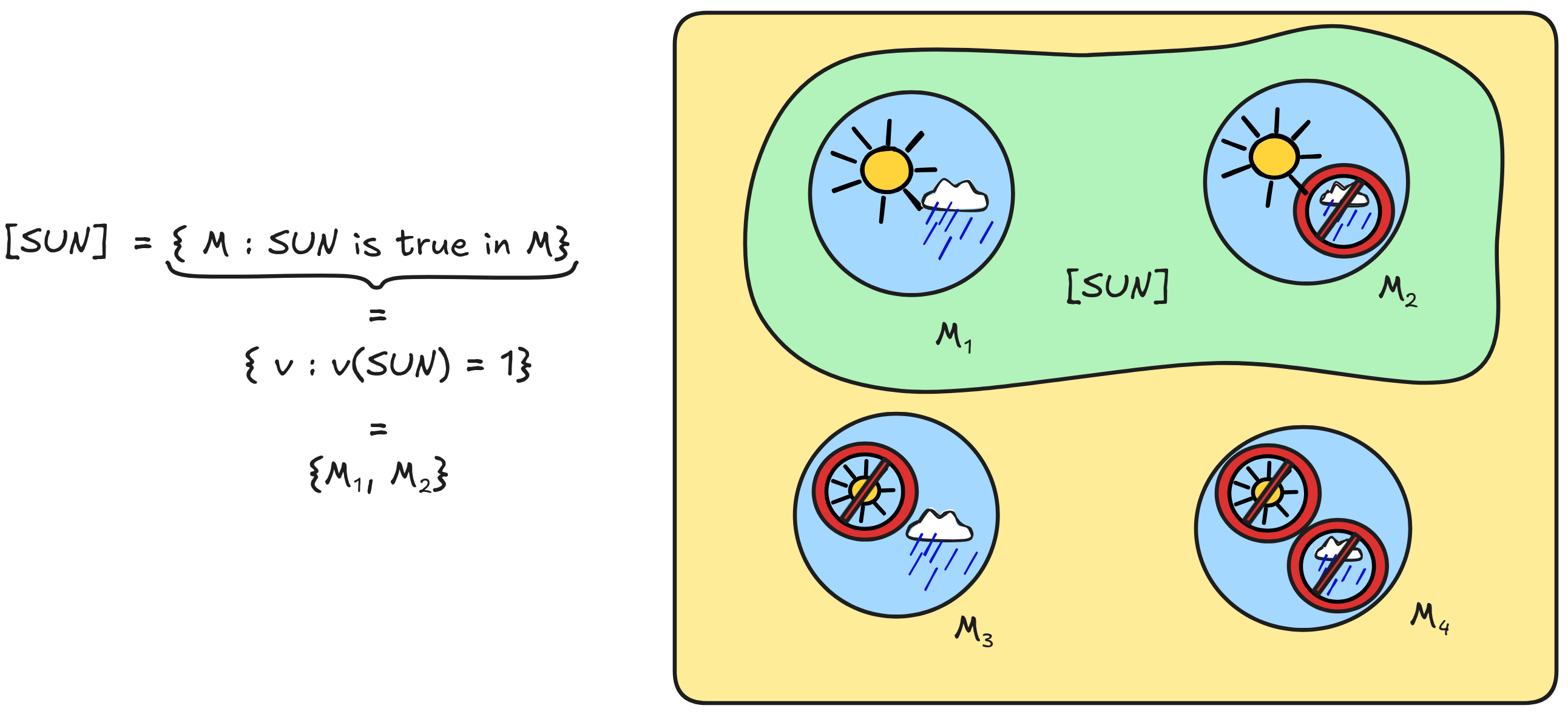
The idea is to identify the possible reasoning scenarios—from a logical perspective—with these assignments. That is, we say that a model for the language L is an assignment of Boolean truth-values to the propositional variables. In short:
Each model tells us what the truth-values for the propositional variables are. This allows as, for example, to determine the proposition [SUN] as follows:
But to determine the truth-values of complex formulas, such as SUN v
RAIN, we first need to think about the connectives. For now, we’ll focus on the connectives
 (“negation”),
 (“conjunction”), and
 .
.
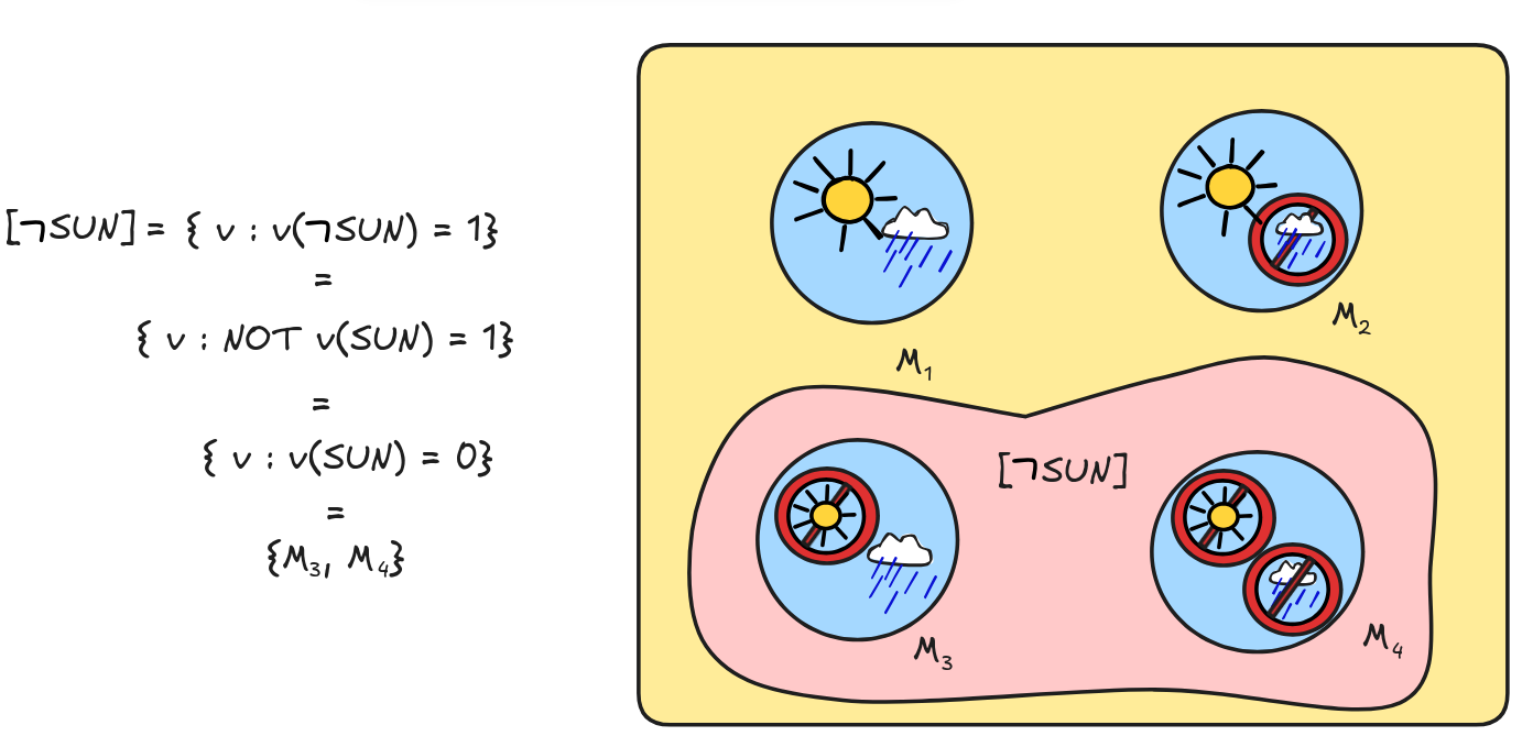
Let’s start with negation. In which models should we say that
 , say, is true? A straight-forward answer
is:
says that it’s not sunny, so the formula
should be true in precisely those models, where SUN is not true:
, say, is true? A straight-forward answer
is:
says that it’s not sunny, so the formula
should be true in precisely those models, where SUN is not true:
) = 1 just in case v(SUN) = 0.But do you recognize it? This is exactly what the Boolean truth-function NOT does! That is, we can implement the proposal using NOT as follows:
) = NOT v(SUN)This means that
gets the following semantic content:
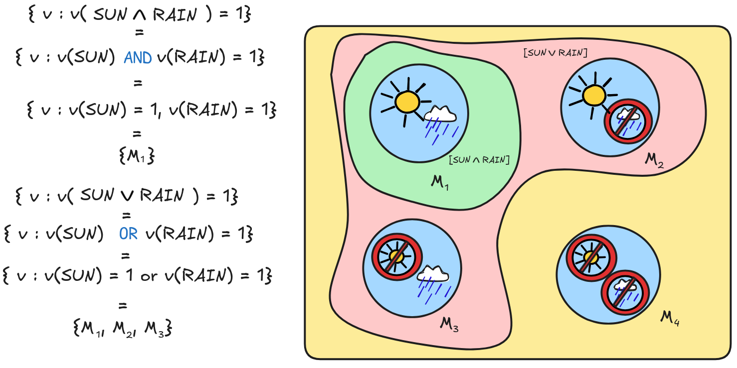
Turning to conjunction, in which models is
 true? Since
the formula says that it’s both sunny and raining, the answer is: precisely in
those models where both SUN and RAIN are true. In all other models,
is false. That is:
true? Since
the formula says that it’s both sunny and raining, the answer is: precisely in
those models where both SUN and RAIN are true. In all other models,
is false. That is:

But that’s just what AND does! So, we can implement this by saying:

Completely analogously, we can handle the case of disjunction.
says that it’s either sunny or rainy. So it should be true in all and only those models where at least one of them is the case.

This we can implement using the Boolean OR by saying that:

In sum,
and
 get the following semantic content:
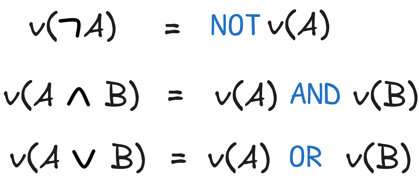
Using this idea, we can calculate the proposition [A] expressed by any formula A of our language. Just apply the following clauses to calculate the truth-values under an assignment:
For example, we can calculate the proposition expressed by
 as follows:
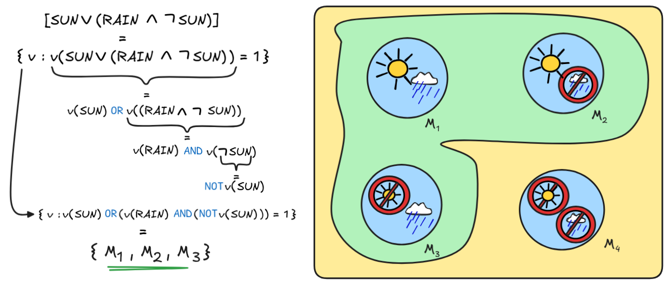
The most difficult part to work out in this example is, as you might have noticed, for which v we have v(SUN) OR (v(RAIN) AND (NOT v(SUN))) = 1. Basically, you need to go through all the valuations and calculate the value of the Boolean expression. This is tedious work! In the next chapter, we’ll discuss methods for making our lives a bit easier using the method of truth-tables for this.
This is, in a nutshell, the standard implementation of the Boolean semantics for propositional logic. Let’s use it to check some inferences for deductive validity!
We’ll do two examples:
-
We’ll show that
 is deductively valid, i.e.

-
We’ll show that
 is deductively invalid, i.e.

The first inference is an instance of Disjunctive Syllogism, which we’ve identified as a paradigmatic example of valid inference. Here, we’ll show that the concrete instance is valid. In the exercises, you’ll show that the general schema is valid for all instances.
To test the inference for validity, what we need to do is to check whether the following condition is satisfied:

So, let’s check in logical space:
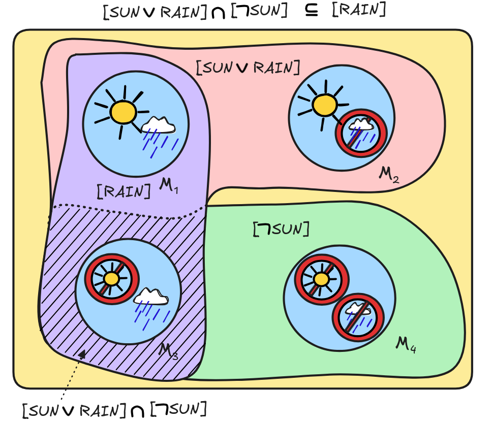
Indeed! Once we’ve worked out the relevant propositions, we can see that the only member of
 is M₄, in which it is raining, i.e. v₄(RAIN) = 1 and so M₄ ∈ [RAIN]. But that just means that our condition is satisfied:
We can conclude that, indeed,
The second inference is an instance of Affirming a Disjunct, which we’ve identified as a traditional fallacy. Let’s see. For the inference to be valid, the following would need to be the case:

When we check logical space, we find the following:
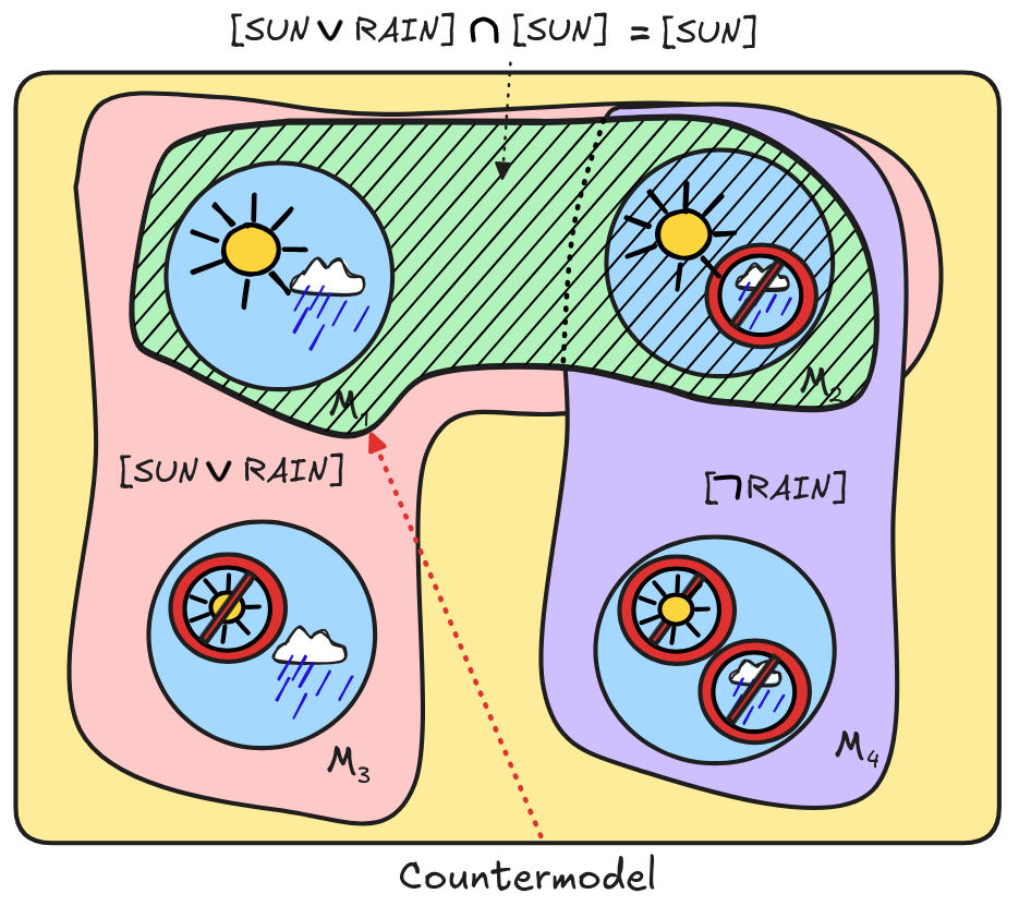
Once we’ve worked out the propositions, we can see that
 . This makes M₁ a countermodel for the inference, which shows that

This means that, indeed:
Note, however, that the invalidity crucially depends on us interpreting
using OR. If we read the operation as an XOR, the story changes—which you’ll see in the exercises.
Further readings
- George Boole’s The Laws of Thought is an enticing historical read.
Last edited: 13/09/2024