Chapter 11
Probability and inductive logic
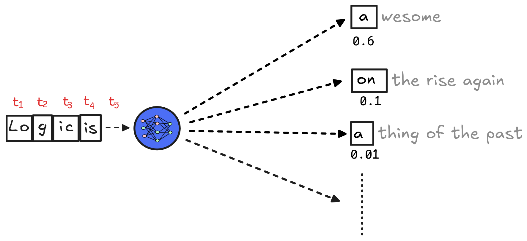 Inductive inference plays a crucial role in AI technologies both on the low
level and on the high level. On the low level, inductive inference is, for
example, the logical foundation for large language models
(LLMs) (opens in a new tab)
, which in turn give
us chatbots (opens in a new tab)
and other modern AI
technologies. In essence, an LLM is (an approximation of) a probability
distribution (opens in a new tab)
over
tokens (opens in a new tab)
—small-ish
sequences of characters that make up words. The idea is that we can use the
conditional probability (opens in a new tab)
of one token given a sequence of others to predict what the next
token in the sequence should be. The perhaps surprising fact is that this
“next-token prediction” allows us to develop AI agents with human-like
abilities.
Inductive inference plays a crucial role in AI technologies both on the low
level and on the high level. On the low level, inductive inference is, for
example, the logical foundation for large language models
(LLMs) (opens in a new tab)
, which in turn give
us chatbots (opens in a new tab)
and other modern AI
technologies. In essence, an LLM is (an approximation of) a probability
distribution (opens in a new tab)
over
tokens (opens in a new tab)
—small-ish
sequences of characters that make up words. The idea is that we can use the
conditional probability (opens in a new tab)
of one token given a sequence of others to predict what the next
token in the sequence should be. The perhaps surprising fact is that this
“next-token prediction” allows us to develop AI agents with human-like
abilities.
 LLMs, and the technologies that they are based on, are the state of the art of
statistics-based AI: they are not based on hand-written if-then rules and
automated deductive inference, but on statistical models of large-scale
datasets, which are developed using advanced machine learning
methods (opens in a new tab)
, such as gradient
descent (opens in a new tab)
. But the fact that LLMs
aren’t
logic-based (opens in a new tab)
doesn’t mean that they have nothing to do with logic. In fact, next-token
prediction is a form of (inductive) inference:
LLMs, and the technologies that they are based on, are the state of the art of
statistics-based AI: they are not based on hand-written if-then rules and
automated deductive inference, but on statistical models of large-scale
datasets, which are developed using advanced machine learning
methods (opens in a new tab)
, such as gradient
descent (opens in a new tab)
. But the fact that LLMs
aren’t
logic-based (opens in a new tab)
doesn’t mean that they have nothing to do with logic. In fact, next-token
prediction is a form of (inductive) inference: t₁, …, tₙ are the previous
tokens, therefore s is the next token. If we want to have any hope at all
of understanding how LLMs work on the low level, we need to study inductive
logic.
 In fact, inference that involves prediction is typically inductive—we can hardly
ever make predictions with certainty. In this chapter, we’ll focus on predictive
inference on the higher, propositional level. As an example of an AI-technology
that features inductive inference we’ll look at
In fact, inference that involves prediction is typically inductive—we can hardly
ever make predictions with certainty. In this chapter, we’ll focus on predictive
inference on the higher, propositional level. As an example of an AI-technology
that features inductive inference we’ll look at SPAM
filters (opens in a new tab)
.
There are different approaches to inductive logic in AI-research. In the logic-based tradition, there are systems which aim to assimilate inductive logic to deductive logic: they work just like the systems we know from deductive logic in terms of syntax, semantics, and proof-theory, except that their consequence relation is inductive: it allows for the premises to be true and the conclusion to be false. The results are systems of non-monotonic logic (opens in a new tab) , such as autoepistemic logic (opens in a new tab) and default logic (opens in a new tab) , which have a solid place in logic-based AI research.
But in broader terms, probability theory (opens in a new tab) is the most widely used framework for inductive logic. In this chapter, we’ll look at probability through the lens of logical theory. As you’ll see, we can develop the standard theory of finite, discrete probability distributions (opens in a new tab) using the truth-tables we’re familiar with from Boolean logic. This allows us to develop the standard theory of inductive inference in the same setting as the standard theory of deductive inference—which in turn makes it possible to compare the two.
Probabilities
Let’s think back to our example of a six-sided die. When we’re rolling the die,
we don’t know what the outcome will be. A process that has different possible
outcomes is called random (opens in a new tab)
in
probability theory. In our case, there are six possible outcomes: we could roll
a 1, a 2, a 3, a 4, a 5, or a 6. Visually, we can represent these possible
outcomes as:
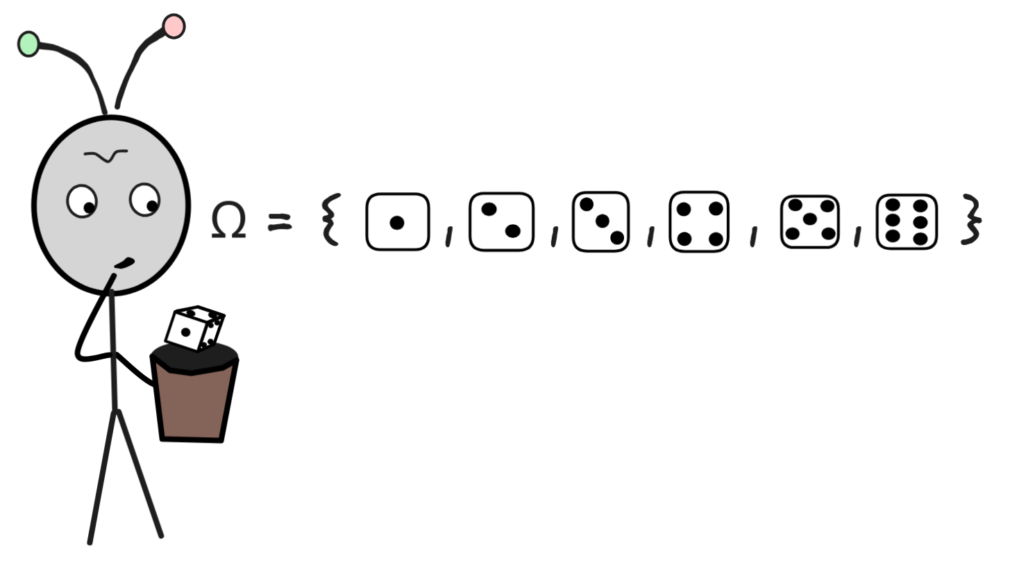 In probability theory, the symbol
 Ω stands for the so-called sample
space (opens in a new tab)
, from which our possible
outcomes are recruited. Rolling the die is what’s called a random
experiment (opens in a new tab)
,
which is a procedure that decides the random process by settling the outcome.
Each outcome in our experiment has a chance of occurring, but what this chance is depends on the die. On a fair die, each outcome is equally likely. On a loaded die (opens in a new tab) , instead, some outcomes are more likely than others. So, there is no “intrinsic” chance that we must assign to the outcomes given our setup of rolling a 6-sided die. There are different possible ways of assigning chances, which correspond to different ways the world could be like.
Formally, we model these different probabilities using what’s called a
probability mass
function (opens in a new tab)
, which is
often denoted p. This is a mathematical function that assigns a value between
0 and 1 (inclusive) to each of our outcomes to measure its chance of
occurring. The value 0 means that it’s impossible for the outcome to occur,
and the value 1 means that it’s absolutely certain. Intermediate values
measure the chance with a higher value meaning a higher chance.
The only constraint on a probability mass function is that the sum of the values over all outcomes must be one, i.e.
p(
 ) + p(
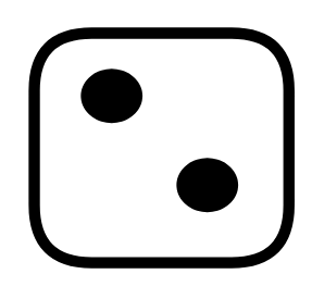 ) + p(
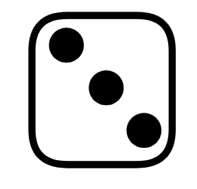 ) +p(
) +p(
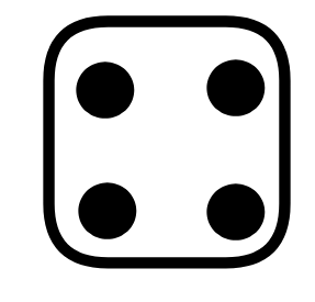 ) + p(
) + p(
) + p(
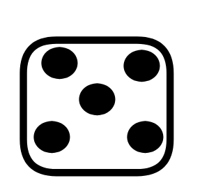 ) + p(
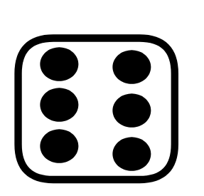 ) = 1
) = 1This constraint captures the idea that at least one of the outcomes must obtain. And behind this way of mathematically expressing this constraint is the idea that the chance of one of a sequence of mutually exclusive outcomes occurring is the sum of the chances of these outcomes. That is, what we’re saying here is that: the chance of the roll either being a 1, a 2, a 3, a 4, a 5, or a 6 is 1—it’s absolutely certain that at least one outcome will occur.
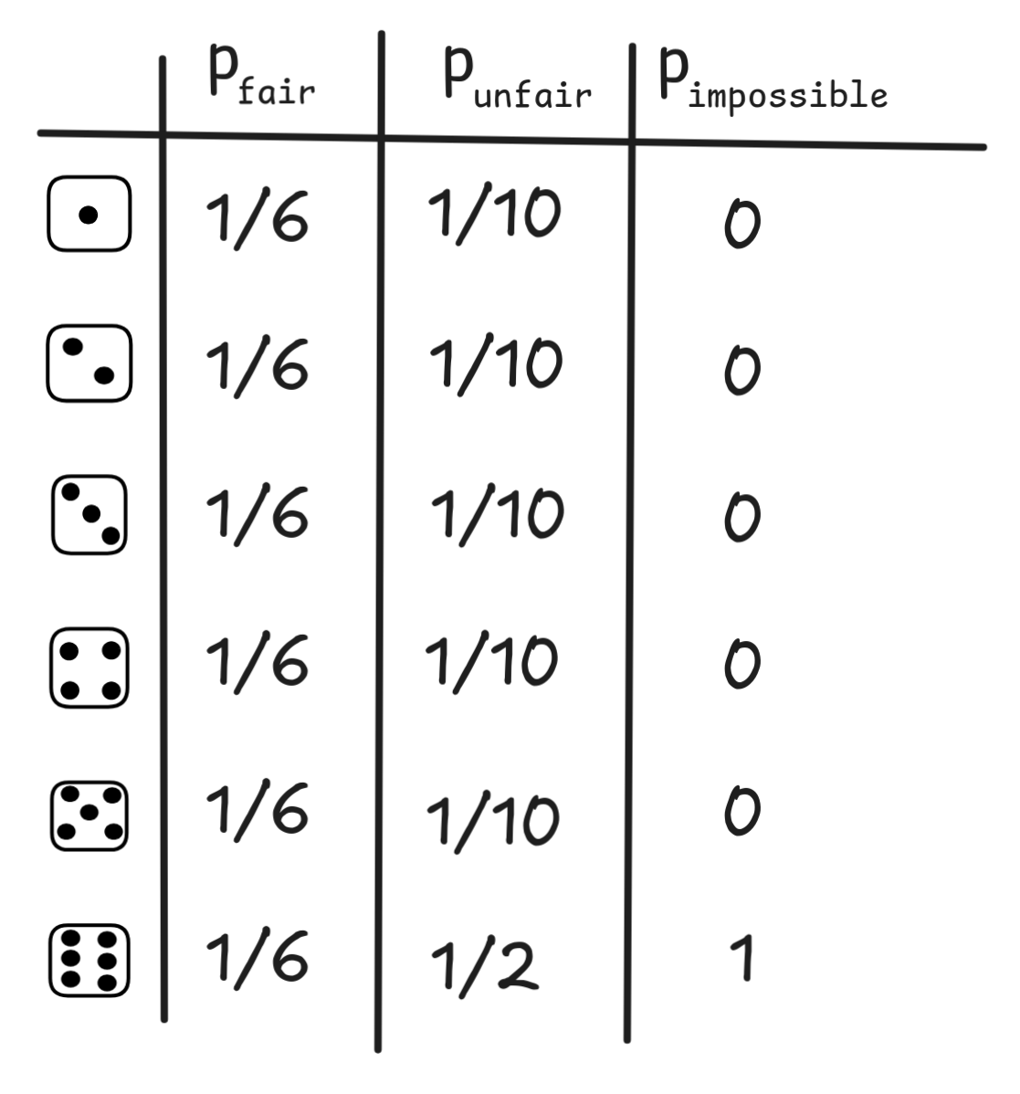
Other than that, any distribution of masses over the outcomes defines a
probability. That is, all of the following are perfectly fine probability
mass distributions:
Once we know the chances of the basic outcomes, we can calculate the probabilities of complex outcomes, like the die showing an even number or showing a number bigger than four. In the parlance of probability theory, these are called events (opens in a new tab) . An event is a set of basic outcomes, the basic outcomes which correspond to the event. So, for example, the event that the die shows an even number is:
{

,

,

}{
,
}To calculate the probability of an event, we simply sum up the probability masses of its outcomes. So, for example,
Pr({

,

,

}) = p(

) + p(

) + p(

)
This probability, then, will differ for each mass function. For our fair die,
e.g., we get Pr({
. But for the unfair distribution, we get
,
,
}) = 1/6 + 1/6 + 1/6 =
3/6 = 1/2Pr({
. Since each outcome
,
,
}) = 1/10 + 1/10 + 1/10 = 3/10ω ∈Ω corresponds to a singleton event, viz. {ω}, we can also write things
like Pr(
, which technically would be
)Pr({
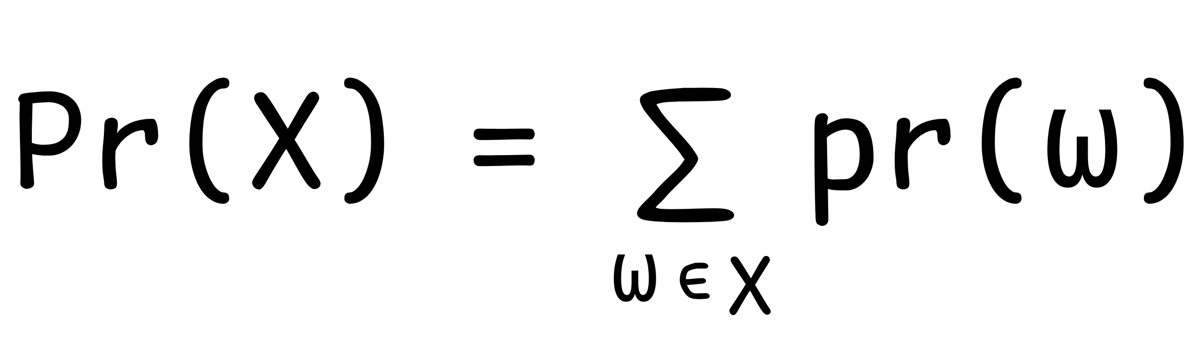
. More generally, the formula for the probability of an arbitrary
event
}) = p(
)X ⊆ Ω is:
This is, in a nutshell, the standard model of (finite) discrete
probabilities (opens in a new tab)
.
Things get a bit more complicated if we want to allow for non-discrete
continuous (opens in a new tab)
values: where the outcomes cannot be counted like 1, 2, 3, … but are things
like real-valued functions with values in an interval [0, 1]. But for the
purposes of basic AI-applications, discrete probability theory is more than
enough.
There is a big debate on the foundations of probability theory concerning what probabilities are:
-
for Bayesians (opens in a new tab) probabilities are a measure of one’s degree of belief in something happening;
-
for frequentists (opens in a new tab) , probabilities measure how often an event would occur if we’d repeat the experiment infinitely many times;
-
for objectivists (opens in a new tab) probability is something “in the world”: just like there’s the mass of an object, there’s the chance of it behaving a certain way.
For our purposes, however, the interpretation of probabilities is not crucial. To explore the relation between probabilities and inductive inference in AI, we can take a naive view of probabilities as chances or likelihoods of something happening.
Note that the outcomes of a random experiment are nothing different than the
reasoning scenarios we’ve discussed in logical semantics. Suppose, for example,
that rather than a die roll, our random experiment is given by tomorrow’s
weather with respect to sun and rain. In this setup, there are four possible
outcomes:

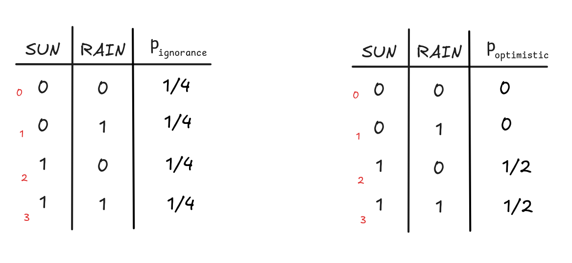
But these are just the models for the propositional language with SUN and
RAIN. In fact, we can think of a probability mass function as an assignment of
values between 0 and 1 to the models of this language. A convenient way of
displaying them is by means of a probabilistic truth-table, which next to
the truth-values, gives the probability of a given row. Here are, for example, two
probabilistic truth-tables: one table that represents a situation where we don’t know
what’ll happen tomorrow, where each outcome is equally likely, and one table
that represents a situation where we know that the sun will shine but it’s
uncertain whether it will rain or not:
Given a probability mass function over the models of a language, we can
calculate the probabilities of arbitrary formulas by calculating the probability
of the proposition they express. Remember that the proposition
⟦A⟧ expressed by a formula A is simply the
set of models where the formula is true:
⟦A⟧ = { v : v(A) = 1 }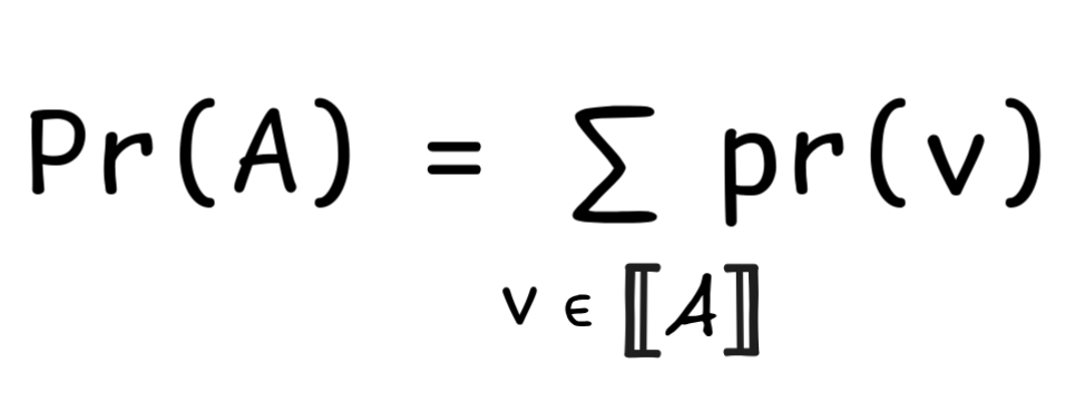
That is, to determine the probability of a formula given a probability mass function, we sum up the masses of all the valuations under which the formula is true.
Truth-tables are of great help here: if you have a probabilistic
truth-table—like the ones above—you can simply calculate the values of your
formula in question for each row, and then sum up the weights of the rows where
the outcome is 1. Here’s how this works out for our two examples and the
formula SUN∨¬RAIN:
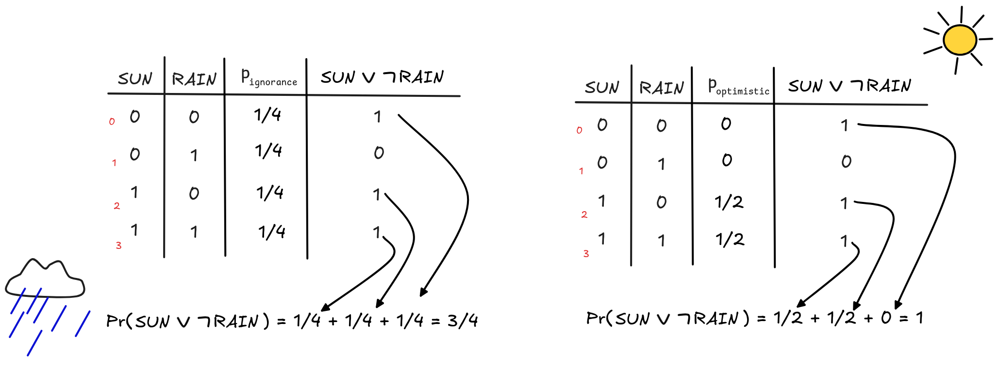 In this way, given a probability mass, we can calculate the probability of each
formula.
In this way, given a probability mass, we can calculate the probability of each
formula.
There’s a crucial difference between truth and probabilities, which is
important to pay attention to. The truth-values of complex formulas are
calculated
recursively (opens in a new tab)
,
which means step-by-step from the values of their parts. The probabilities of
complex formulas, however, are not (in general) recursive. Take, for example,
the probability of SUN∧RAIN under the ignorance distribution and compare
it to the probabilities of SUN and RAIN:
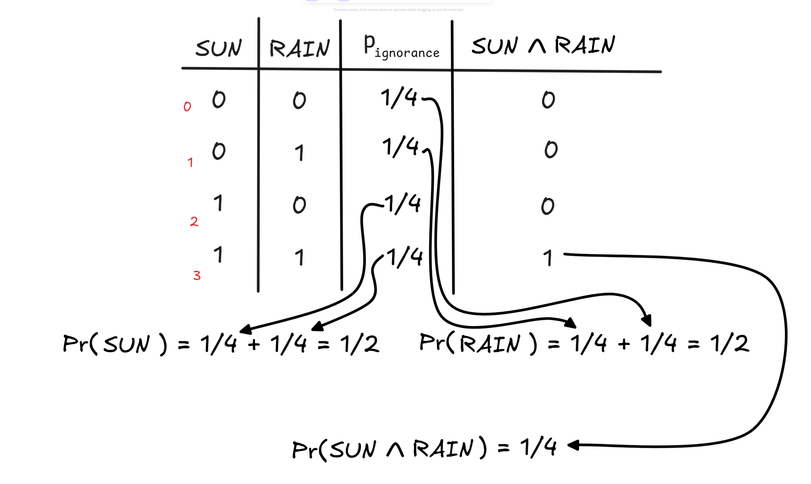
With this probability mass distribution, we have that
Pr(SUN∧RAIN) = PR(SUN) x Pr(RAIN)But this formula doesn’t apply under all distributions. Look, for example, at
the following table with the distribution p*:
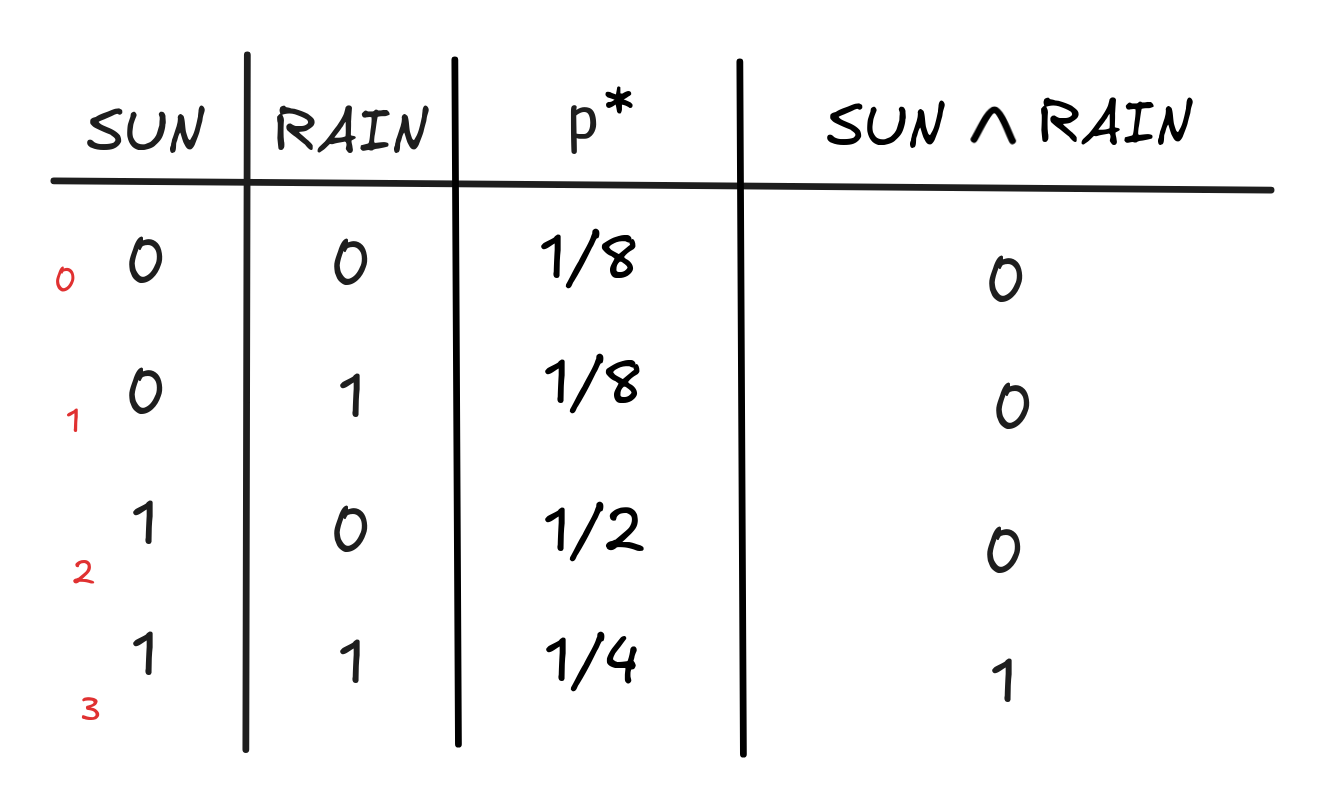
This table represents a situation where it’s more likely to be sunny than not. We have:
Pr(SUN) = 1/2 + 1/4 = 3/4If we’re looking at the situations where the sun shines, it’s relatively
unlikely that it will rain: the world where the sun shines and it’s not raining
has probability 1/2 and the one where the sun shines and it’s raining has
probability 1/4.
If instead, we look at the two situations where the sun
isn’t shining, we see that it’s equally likely among those that it’s raining:
both scenarios, sun and rain as well as sun and no rain, have probability
1/8. The probability that it’s raining is therefore:
Pr(RAIN) = 1/8 + 1/4 = 3/8But if we look at the probability of the conjunction, we get that:
Pr(SUN∧RAIN) = 1/4And clearly, 1/4 is different from 3/4 x 3/8 = 9/32. In fact, there is no
formula that allows us to calculate the probability of a conjunction purely on
the basis of the probabilities of its conjuncts.
What’s going on here has to do with probabilistic independence (opens in a new tab) . In the first distribution, the two facts that it’s raining and that the sun is shining are independent of each other: under the distribution, knowing that the sun is shining, this doesn’t have any influence on the probability of it raining.
To further illustrate this, we can use the concept of conditional probabilities (opens in a new tab) .
We’ve already seen the definition of conditional probabilities in terms of propositions when discussing valid inference:
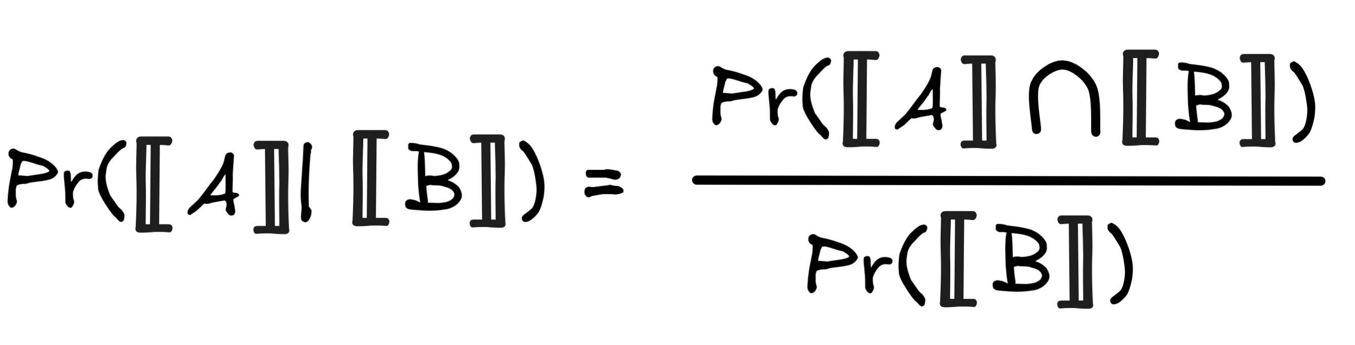
Here, the crucial condition that Pr(⟦B⟧) ≠ 0 applies. But using the following identity:
⟦A∧B ⟧ = ⟦A ⟧∩⟦B ⟧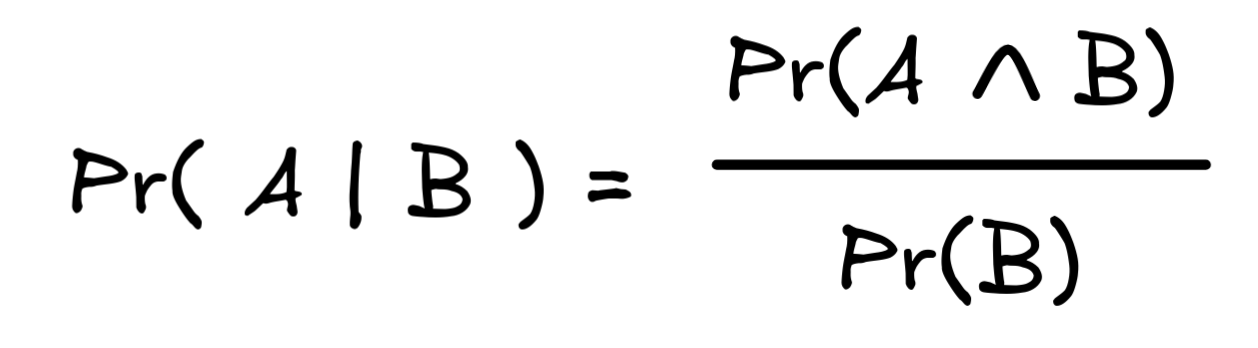
Now look at what happens in the case of our ignorance distribution, if we
calculate Pr(RAIN | SUN). First, we note that:
Pr(RAIN) = 1/4 + 1/4 = 1/2 Pr(SUN) = 1/4 + 1/4 = 1/2Pr(SUN ∧RAIN) = 1/4Pr(RAIN | SUN). We get:
Pr(RAIN | SUN) = Pr(SUN ∧RAIN)/Pr(SUN) = (1/4)/(1/2) = 2/4 = 1/2Pr( RAIN | SUN ) = Pr(RAIN)If we look at the distribution p*, instead, we get:
Pr(SUN) = 3/4 Pr(RAIN) = 3/8Pr(SUN ∧RAIN) = 1/4And so, we have that:
Pr(RAIN | SUN) = Pr(SUN ∧RAIN)/Pr(SUN) = (1/4)/(3/4) = 4/12 = 1/3That means that under the hypothesis that it’s sunny, the probability of rain
changes—in fact, it goes down (since 1/3 < 3/8).
Two formulas A and B are said to be probabilistically independent just
in case they are like SUN and RAIN in our first distribution, that is
just in case
Pr(A | B) = Pr(A)In the case where A and B are probabilistically independent, we have
Pr( A ∧B ) = Pr(A) x Pr(B)Pr(A | B) = Pr(A). By the formula for conditional probabilities, we
have that Pr(A | B ) = Pr(A ∧B)/Pr(B). So, if we multiply
by Pr(B), we get Pr(A | B) x Pr(B) = Pr(A ∧B). But since
Pr(A | B) = Pr(A) by assumption, we have that Pr(A) x Pr(B) = Pr(A
∧B).
In fact, this is a test for probabilistic independence as well: if
Pr(A ∧B) = Pr(A) x Pr(B), then Pr(A | B ) = Pr(A). This
is simply because Pr(A | B) = Pr(A ∧B)/Pr(B). So, if Pr(A
∧B) = Pr(A) x Pr(B), we have that:
Pr(A | B) = Pr(A ∧B)/Pr(B) = (Pr(A) x Pr(B))/Pr(B)= Pr(A)In the absence of independence, the best thing we can say about the probability of a conjunction is that:

This covers conjunction. Disjunction is subject to similar considerations. Take
our ignorance table and look at the disjunction SUN ∨RAIN:
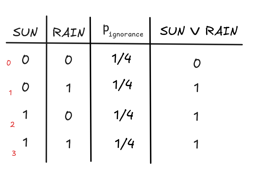
We get:
Pr(SUN ∨RAIN) = 1/4 + 1/4 + 1/4 = 3/4Here we’re adding the probabilities of three different scenarios: sun without rain, rain without sun, and both sun and rain. These scenarios don’t overlap, so we can simply add their probabilities.
But adding Pr(SUN) and Pr(RAIN) would count the last scenario twice: once
as a sunny scenario and once as a rainy one. We need to subtract its probability
once to correct for that double counting. In our example, this gives
1/2 + 1/2 - 1/4 = 3/4.The same reasoning gives the general formula for a disjunction:
Pr(A ∨B) = Pr(A) + Pr(B) - Pr(A ∧B)But that means that, in general, we cannot calculate the probability of a disjunction from the probabilities of its disjuncts—we also need to know the probability of their conjunction.
Only in the very special case where Pr(A ∧B) = 0, when A and B
are probabilistically incompatible, we get the recursive formula:
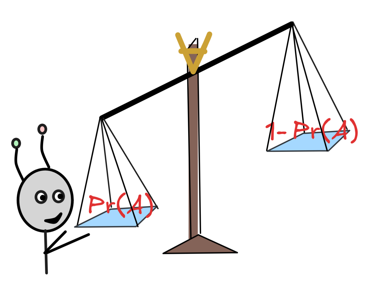
Pr(A ∨B) = Pr(A) + Pr(B)The only case where we have a full recursive rule is the case of negation. Under each distribution, we have
Pr(¬A) = 1 - Pr(A)A is true are precisely the rows where
¬A is not, and the masses of the rows add up to 1.
Probability Laws
 The fact that probabilities aren’t recursive puts special
emphasis on the laws of probability. Moreover, in AI research, you’re often
dealing with situations where it’s practically
intractable (opens in a new tab)
to go through all possible models of the premises and assign them probability masses.
Instead, you’ll be estimating the relevant probabilities of the formulas
directly. And when you do that, you have to make sure you’re doing this in
accordance with the laws of probability.
The fact that probabilities aren’t recursive puts special
emphasis on the laws of probability. Moreover, in AI research, you’re often
dealing with situations where it’s practically
intractable (opens in a new tab)
to go through all possible models of the premises and assign them probability masses.
Instead, you’ll be estimating the relevant probabilities of the formulas
directly. And when you do that, you have to make sure you’re doing this in
accordance with the laws of probability.
The standard axiomatization of probability is due to Andrey Kolmogorov (opens in a new tab)
and correspondingly
known as the Kolmogorov
axioms (opens in a new tab)
. We can formulate these
axioms in logical terms and directly in terms of events. First, the logical
axiomatization. It states that for each assignment of probabilities Pr to
formulas in a language, the following laws apply:
Pr(A) ≥ 0, for all formulasA.Pr(A) = 1, ifAis a tautology, that is:⊨ A.Pr(A ∨ B) = Pr(A) + Pr(B), given thatAandBare logically incompatible, that is:⊨ ¬(A∧B).
As you can see, these axioms are rather minimal. But it turns out that they are
sound and complete with respect to the probabilities we’ve defined in terms of
probability mass distributions over valuations. That is, every law about
probabilities that holds for all probabilities Pr defined in terms of
probability mass distributions is derivable from these laws, and everything
that’s derivable holds for all distributions.
For example, here’s how we derive the law of negation:
Pr(¬A) = 1 - Pr(A) ("Negation")Pr(A ∨¬A) = 1, by axiom 1. since⊨A∨¬A.Pr(A ∨¬A) = Pr(A) + Pr(¬A)by axiom 3. since⊨¬(A ∧¬A).- It follows that
1 = Pr(A) + Pr(¬A). - But that gives us:
Pr(¬A) = 1 - Pr(A)
From this it immediately follows that Pr(A) ≤ 1 for all A, since Pr(A) = 1
- Pr(¬A).
Or, we can derive that if A⊨B, then Pr(A) ≤ Pr(B):
Pr(A ∨ ¬B) = Pr(A) + Pr(¬B), by axiom 3., since from the assumption thatA⊨Bit follows that⊨¬A∧¬B—that is ifAand¬Bis unsatisfiable.- Since
Pr(¬B) = 1 - Pr(B), we havePr(A ∨ ¬B) = Pr(A) + (1 - Pr(B)). - So, we get that
Pr(B) = Pr(A) + (1 - Pr(A ∨¬ B)). - But we know that
Pr(A∨¬B) ≤ 1, so1 - Pr(A ∨¬ B)is positive and soPr(B) = Pr(A) + x, for some positivex. - In other words,
Pr(A) ≤ Pr(B).
We can give these axioms completely equivalently directly in terms of events:
0≤Pr(X), for all eventsX ⊆ ΩPr(Ω) = 1Pr(X ∪Y) = Pr(X) + Pr(Y), given thatX∩Y = ∅.
This axiomatization says precisely the same thing as the previous one once we
realize that ⟦A⟧ = Ω means that A is a
logical truth and
⟦A ∨B⟧ = ⟦A ⟧∪⟦B ⟧Naive Bayes Classifiers
To see how AI-technologies use probabilities for inductive inferences, let’s look at an example: spam filtering (opens in a new tab) with naive Bayes classifiers (opens in a new tab) .
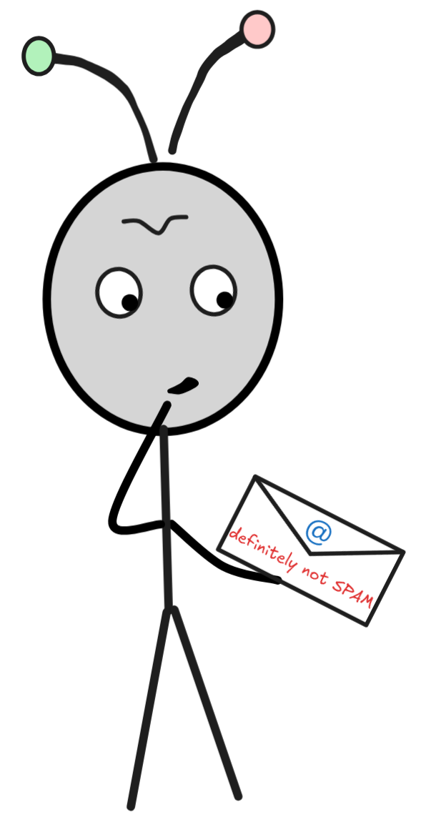
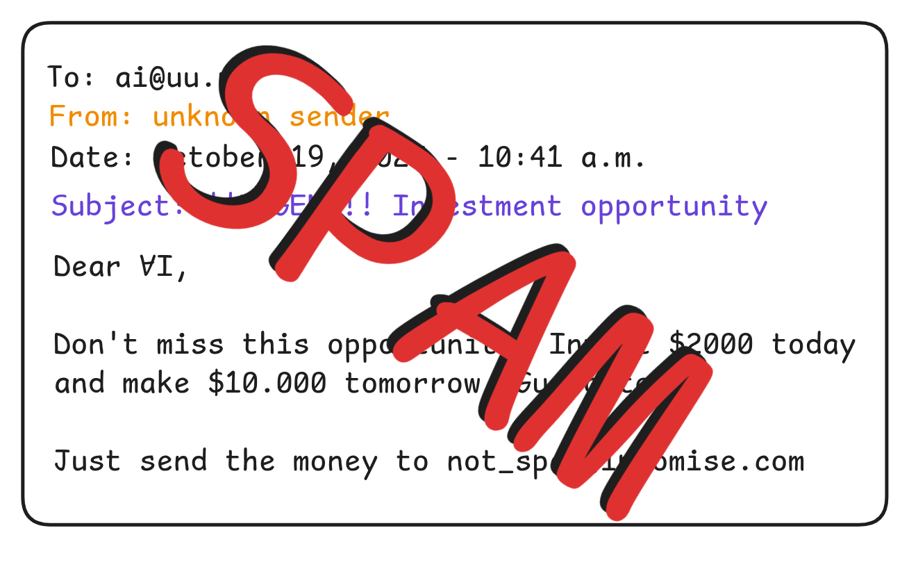
For our example, let’s suppose that receives an email:
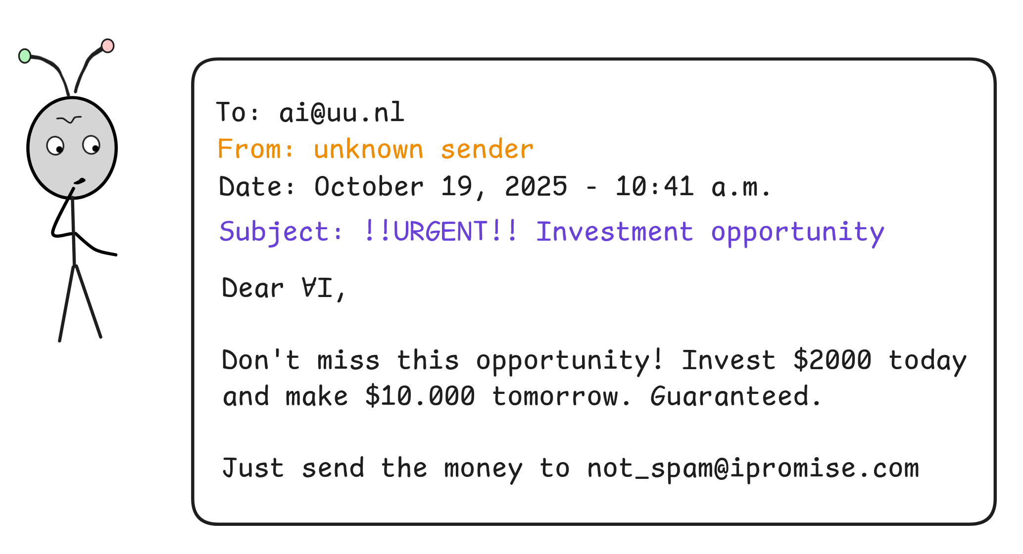
How can
tell that this is a SPAM email?
Since we’re in a logic course, you might think that we’d try to develop an expert system for this task. We devise a propositional language with atoms like
UnknownSender, SubjectUrgent, ExclamationMarks, MoneyTalk, SPAMIn this language, we can formulate conditional rules like:
(SubjectUrgent∧MoneyTalk) → SPAM(ExclamationMarks∧SubjectUrgent) → SPAM…
Then we could run a filter through each email and check whether the propositions
UnknownSender, SubjectUrgent, ExclamationMarks, MoneyTalk are true and use the
KB to see if we can derive SPAM using methods like forward chaining or
backward chaining or resolution.
But the problem with this approach is that none of these indicators are 100% reliable. We can have an email that satisfies all of them but is perfectly harmless:
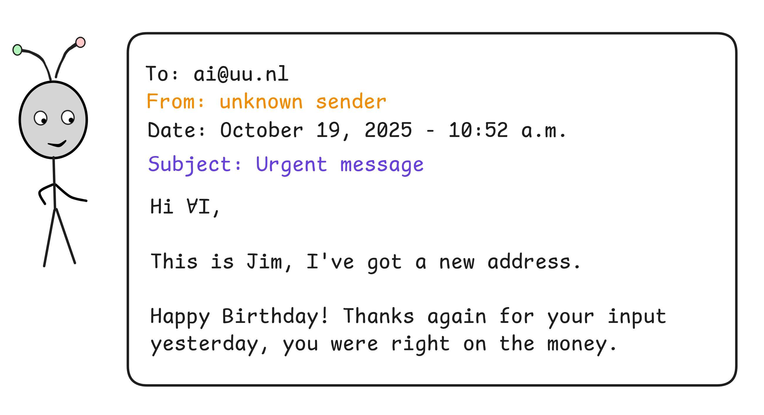
That is, using deductive inference will lead to a lot of false
positives (opens in a new tab)
.
In fact, the conditions that we’ve mentioned aren’t logically
sufficient (opens in a new tab)
for an
email being SPAM, they are fallible
evidence (opens in a new tab)
for it.
A powerful approach to inductive inference uses probabilities and Bayes'
rule (opens in a new tab)
. The basic idea is that we
can say that a piece of propositional evidence, E, confirms a hypothesis, H,
just in case:
Pr(H | E) > Pr(H)So, what we’re looking for is Pr(SPAM | [MARKERS]), where [MARKERS]
is a combination of things like UnknownSender, SubjectUrgent, ExclamationMarks,
MoneyTalk. That is, to see whether the present markers are evidence for the mail being
SPAM, we need to calculate Pr(SPAM | [MARKERS]) as well as Pr(SPAM).
Bayes rule is, in essence, a convenient way of calculating Pr(SPAM | [MARKERS]):
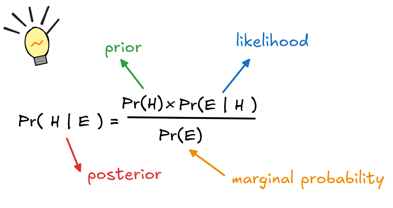
This calculation is derived by simply substituting P(H ∧E) with
Pr(H) x Pr(E | H) from the general rule for conjunction. The terms in the
equation have suggestive names:
-
Pr(H | E)is known as the posterior probability (opens in a new tab) of the hypothesis given the evidence. -
Pr(H)is called the prior probability (opens in a new tab) of the hypothesis, independent of the evidence. -
Pr(E | H)is known as the likelihood (opens in a new tab) of the evidence given the hypothesis. -
Pr(E)is known as the marginal likelihood (opens in a new tab) of the evidence.
Plugging in SPAM and [MARKERS], we obtain:

This is progress: the prior probability, Pr(SPAM), we can estimate using the
frequency of SPAM (opens in a new tab)
. For this example,
let’s estimate it optimistically as 20%. In probabilistic terms:
Pr(SPAM) = 0.2For individual markers, like UnknownSender, SubjectUrgent, ExclamationMarks,
MoneyTalk, we have to estimate the marginal likelihood Pr([Markers]) and
likelihood Pr([Markers] | SPAM). In practice, this happens on the basis of
a frequency analysis of datasets of emails, especially the ones you have
received. For each marker, we can easily check how often it occurs in an email:
how many emails are from unknown senders, how many emails have “urgent” in the
subject line, and so on. Dividing these numbers by the total number of emails
gives us a decent estimate of their respective probabilities. We might, for
example, find:
Pr(UnknownSender) = 0.3Pr(SubjectUrgent) = 0.4Pr(ExclamationMarks) = 0.6Pr(MoneyTalk) = 0.3The same procedure, we can use to estimate the likelihoods for the markers given
in SPAM messages. What’s the frequency of SPAM emails with an unknown sender,
SPAM emails with an urgent subject line, etc. For example, we might find:
Pr( UnknownSender | SPAM ) = 0.4Pr( SubjectUrgent | SPAM ) = 0.6Pr( ExclamationMarks | SPAM ) = 0.7Pr( MoneyTalk | SPAM) = 0.6We can plug this data into Bayes rule and obtain estimates of how likely it is
that an email is SPAM given that it comes from an unknown sender:
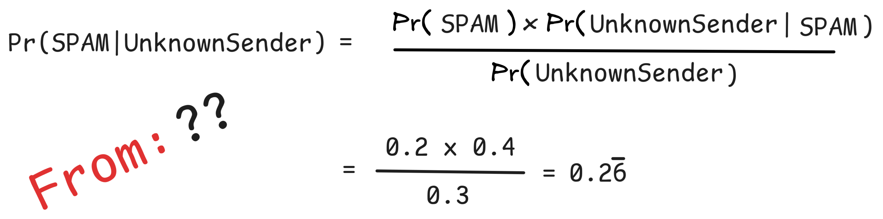
Since
Pr(Spam | UnknownSender) = 0.26 > 0.2 = Pr(Spam)receiving an email from an unknown sender is evidence of it being SPAM—but
not very strong evidence.
What does this mean? Well, for one, the probability of the email being SPAM
only went up by 0.06. This is the so-called increase of firmness measure
incOfFirmness(E, H) = |Pr(H | E) - Pr(H)|In our case, the increase of firmness is not very strong.
But note that the probability of the email being SPAM went up from 0.2 to
0.26, which is a 30% increase. This is known as the ratio measure:
ratioStrength(E, H) = Pr(H | E)/Pr(H)There are many more such confirmation measures. In fact, in industry implementations of naive Bayesian classifiers the so-called log-likelihood ratio (opens in a new tab) is commonly used, but we won’t go into the more involved mathematical details here.
Different measures have different advantages: for example, the increase of firmness gives an intuitively clear and robust measure of strength of evidence, but it doesn’t work very well with evidence and hypotheses close to 0 or 1. The ratio measure, instead also works well close to extreme values, but it is not normed (opens in a new tab) —in particular its value can get arbitrarily high making comparisons difficult.
But regardless of different measures of how much weight the evidence carries,
there’s another fundamental question we’ve got to address: if the posterior
probability is “only” 0.26, it’s still more likely that this isn’t SPAM than
that it is. What we need to do is to set a
threshold (opens in a new tab)
for classifying email
as SPAM. A natural minimum is to say that Pr(H | E) should at least be
0.5. But if false
positives (opens in a new tab)
are particularly bad—when classifying email as SPAM that isn’t risks important
messages being missed—we should set the bar high. Perhaps we want to have 0.75?
0.8? It ultimately depends on the stakes of the situation, but let’s try to
reach 0.5 in our SPAM filter.
To achieve this, we need to combine different markers. What we want to
do is to combine different SPAM-markers. In fact, our example mail had them
all. So, we want to calculate:
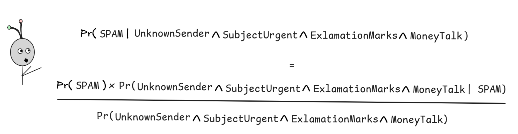
But now we have a new kind of probability to estimate: the conjunctive probabilities of the markers. In fact, we want our classifier to work not only in this case, but also when one or more of the markers are absent. But since conjunctive probabilities are not recursively calculable from their conjunctions’ probabilities, this leads to a problem of combinatorial explosion (opens in a new tab) In our example, we only have 4 markers, but that’s already quite a large number of conjunctions to estimate: all 4 markers by themselves, their 6 binary conjunctions (up to re-ordering), their 4 ternary conjunctions, and the conjunction of all 4 makes 15 conjunctions we need to estimate. This quickly becomes intractable.
This is where the “naive” in naive Bayes classifiers comes in. The defining
assumption is that the different markers are probabilistically independent of
each other, both given SPAM and not given SPAM. That is, we can calculate:
Pr( UnknownSender ∧ SubjectUrgent ∧ ExclamationMarks ∧ MoneyTalk | SPAM)=Pr(UnknownSender | SPAM) x Pr(SubjectUrgent | SPAM) x ...... x Pr(ExclamationMarks | SPAM) x Pr(MoneyTalk | SPAM)And similarly,
Pr( UnknownSender ∧ SubjectUrgent ∧ ExclamationMarks ∧ MoneyTalk)=Pr(UnknownSender) x Pr(SubjectUrgent) x ...... x Pr(ExclamationMarks) x Pr(MoneyTalk)This, then is the naive Bayes assumption: that the different markers are conditionally independent. It is naive because it is clearly false in strict terms: whether urgent and exclamation points occur is not independent of each other. But it turns out that this gives us pretty good classifications in practice. It gives us for our email:
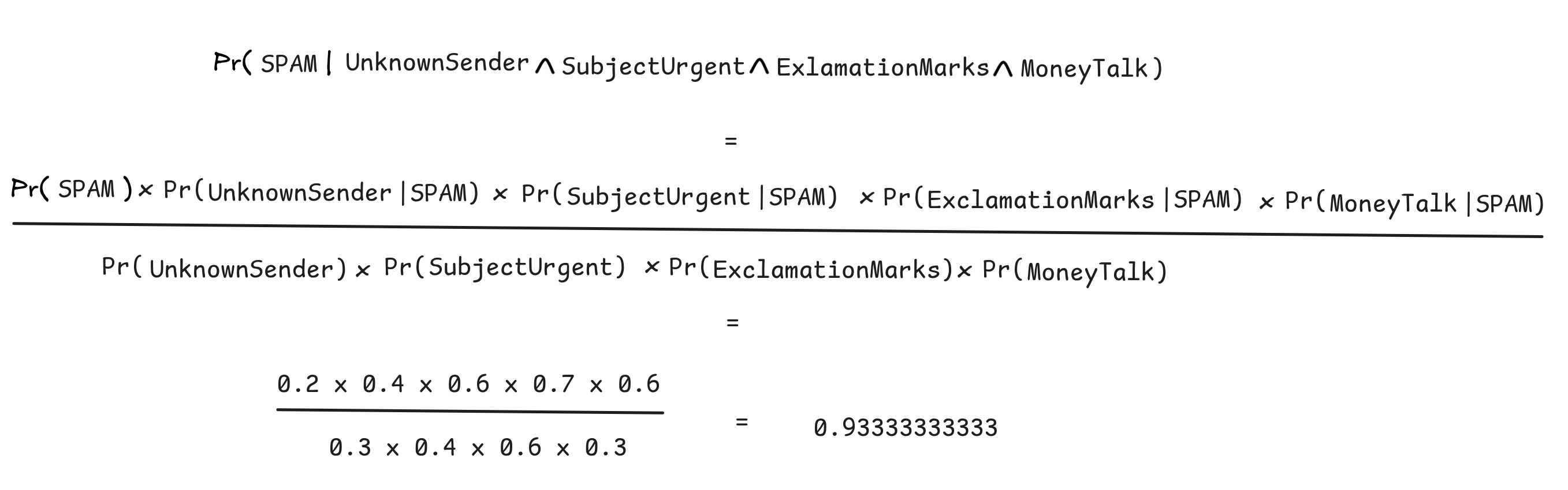
A pretty clear verdict, which surpasses any reasonable threshold: we’ve got a strong inductive inference that this is spam, given the observed features.
But it also allows us to quickly estimate the SPAM likelihood of other emails.
For example, if the exclamation marks are absent, the formula would still give a
0.8 probability of SPAM given that the other features are still present. But
if money talk is eliminated, the probability drops down to 0.46. Fine-tuning
these values, checking them against real cases and learning from data is the
topic of ongoing machine learning research.
Inductive logic
SPAM-classification is a case of material inductive
inference (opens in a new tab)
: what counts as a
good inductive inference depends on the concrete (conditional) probabilities of the premises
and conclusion. Logically valid inductive inference is inductive inference that
purely depends on their logical form. We can cash this out as probability
raising under all probabilities:
P₁, P₂, ...
 C if and only if for all Pr, we have Pr(C | P₁ ∧ P₂∧ ) ≥ P(C)
Inductive logic is concerned with the study of inductively valid inference patterns. Today, this is mainly done as statistics and probability theory, whose study goes beyond the scope of this course. But we can get a rough idea of some core ideas by returning to one of our first examples of inductive inference: enumerative induction (opens in a new tab) .
Take our inference about the marbles:
All marbles we've observed so far were white∴All marbles are whiteIf we formalize this inference with a sufficient number of observations, we’ll look at something like:
White m₁, ..., White mₙ ∴∀x White xTo assess the logical validity of this inference, we need to think about the conditional probability independently of any concrete probability distribution:
Pr(∀x White x | White m₁∧ ...∧ White mₙ)For this purpose, we can make use of probabilistic theorems like the following:
To see that this must be true, we need to observe the logical fact that:
if C⊨ P₁ ∧ P₂, then ⟦C ∧P₁ ∧ P₂∧...⟧ = ⟦C⟧Using this, we can calculate:
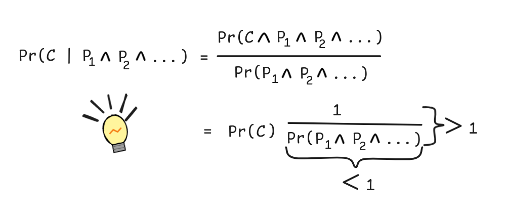
That is, since Pr(P₁ ∧ P₂∧…) < 1, we know that
1/Pr(P₁ ∧ P₂∧…) > 1 and so Pr(C | P₁ ∧
P₂∧…)is more than one timesPr(C)—in other words,Pr(C | P₁
∧ P₂∧…)is strictly bigger thanPr(C).
This establishes that enumerative induction is at least weakly inductively valid: the premises will always raise the likelihood of the conclusion.
The strength of the inference depends on the probability of P₁∧
P₂∧…—the less likely the premises the bigger the factor in the
above equation and, correspondingly, the stronger the inference. This justifies
the condition that we need to sample our premises well—it should be unlikely
that they are jointly true. We can achieve this by finding many independent
instances and calculating Pr(P₁∧ P₂∧…) = Pr(P₁) × Pr(P₂)
× …, which will eventually bring us below any desired threshold.
Inductive reasoning is the ultimate foundation for most machine learning techniques, but also for simple algorithms like “People who liked this show also liked …"-style recommendation on streaming platforms, which makes inductive logic a fundamental tool in an AI-researcher’s toolbox.