Logical conditionals

---

The conditional is the backbone of valid inference. We’ve said that valid inference is based on hypothetical reasoning: valid inference requires that the conclusion be true under the hypothesis that the premises are—if the premises are. This applies to both deductive and inductive inference, but in this chapter, we’ll focus on deductive inference.

The conditional of deductive logic, which we formalize as , is the basis for many artificial reasoning techniques, especially in logic-based AI. It turns out that conditional reasoning is crucial to many AI-related tasks. Think for example of computer code like this: 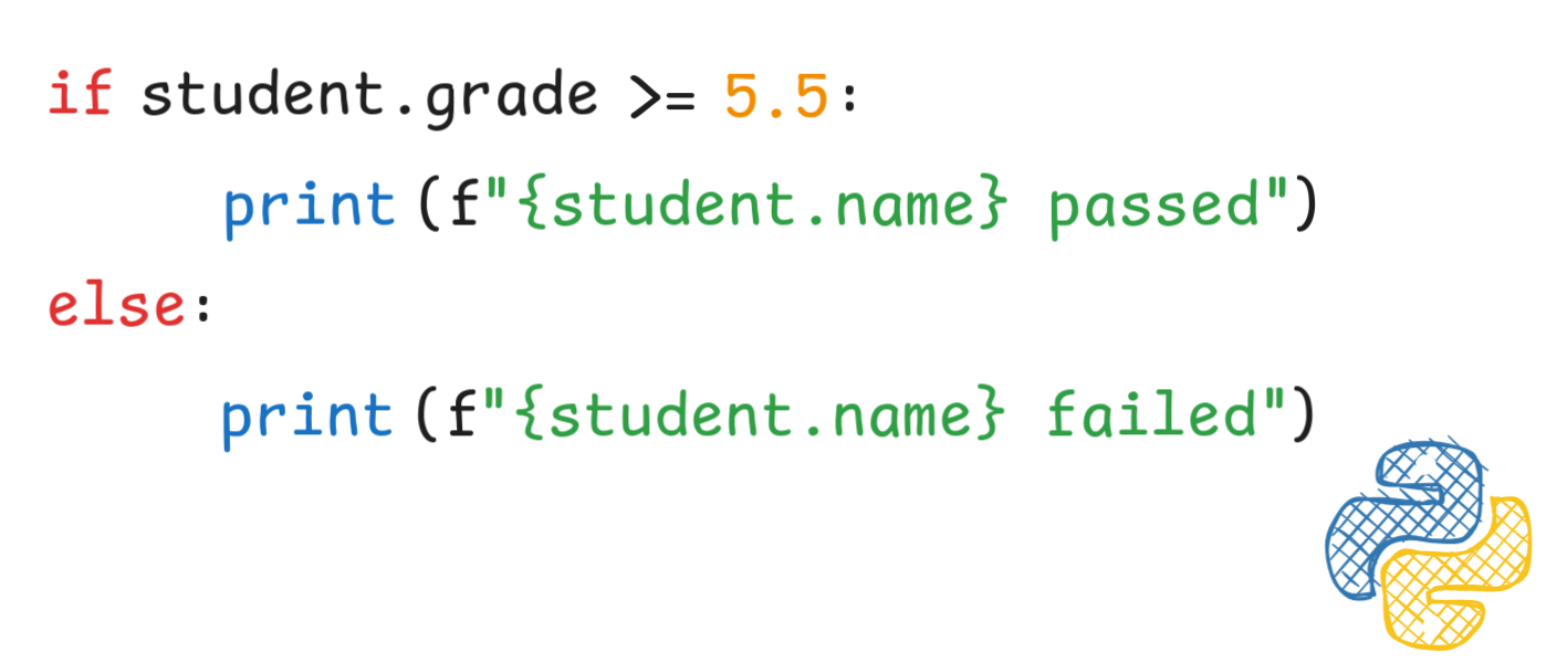Both to evaluate and understand this code, we need to understand basic conditional reasoning.

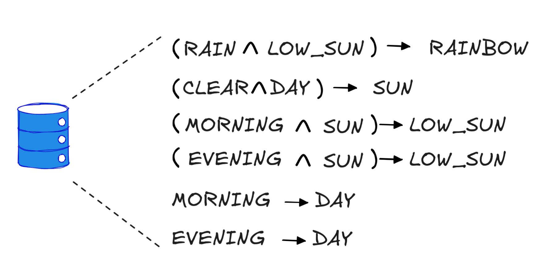
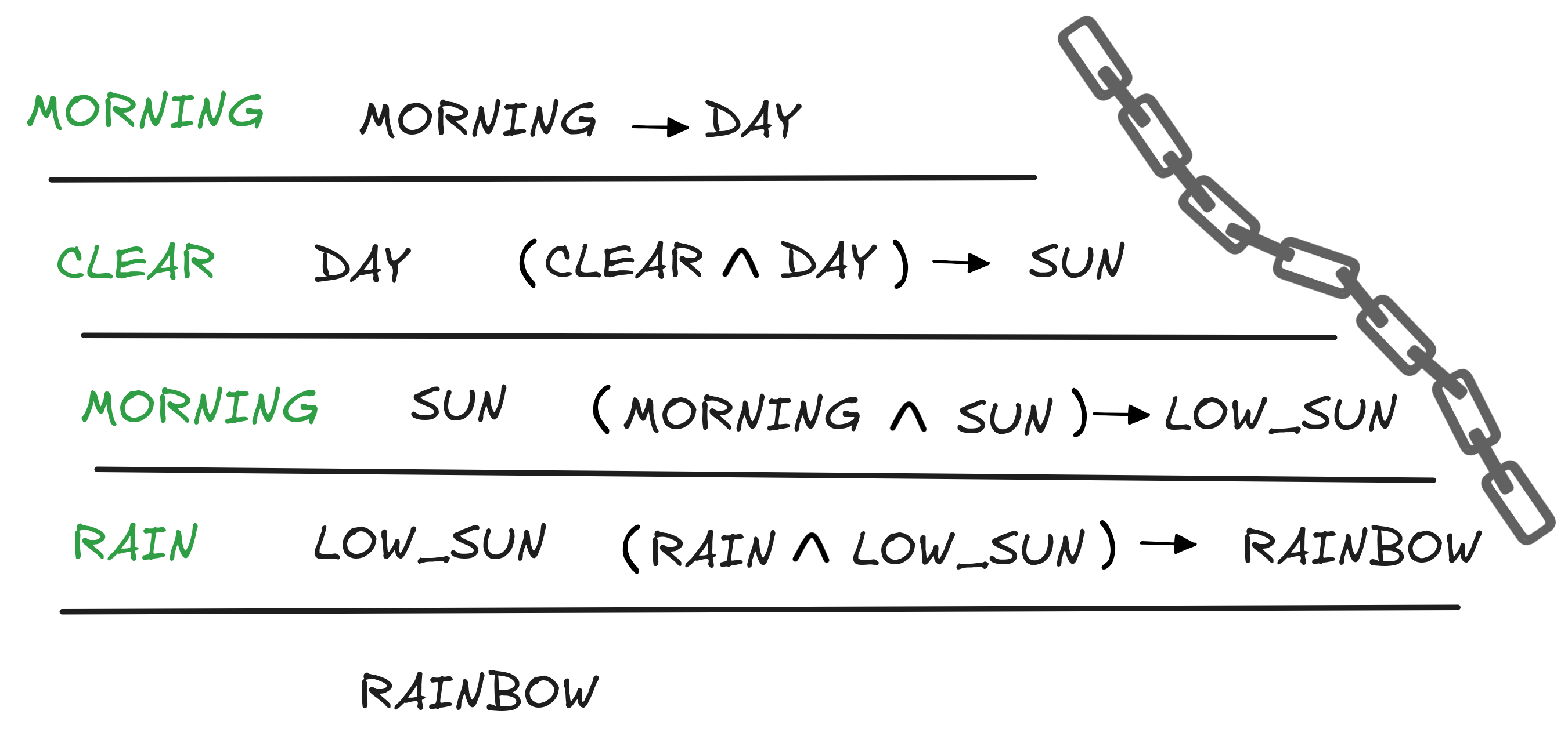
Or, imagine a very simple meteorology KB, which might contain the following information: 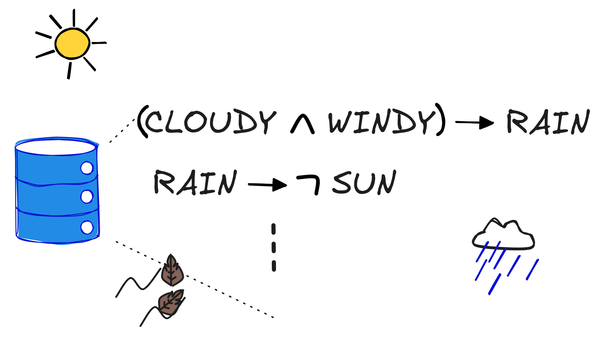If we want to use this information for automated weather forecasting, we need to think about artificial conditional inference. That’s the topic of this chapter.

At the end of it chapter, you will be able to:

• explain the relationship between deductive reasoning and conditionals
• outline the basic theory of the Boolean material conditional and the theory of Horn formulas
• apply basic algorithms for conditional reasoning, such as backward and forward chaining
• use conditionals to formalize rules in knowledge representation scenarios
• explain the limitations of Horn formulas in knowledge representation and reasoning

Boolean If-then

---

The most characteristic inference involving is the principle of Modus Ponens (MP):

How can we develop a theory of conditional logic which validates this principle?

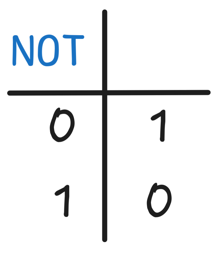
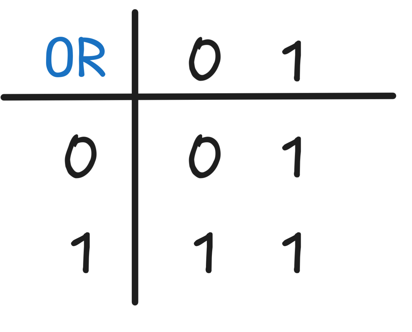
It turns out that Boolean algebra already has the resources to interpret in a way that aligns with many of our expectations about if-then statements. The idea is that we can interpret using the Boolean functions NOT and OR in combination:

The way this works is by saying:

Using this clause, the truth-table for (RAIN WIND), for example, works out to:

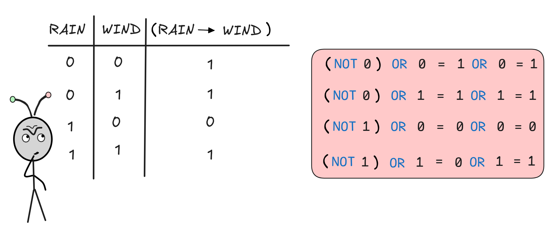
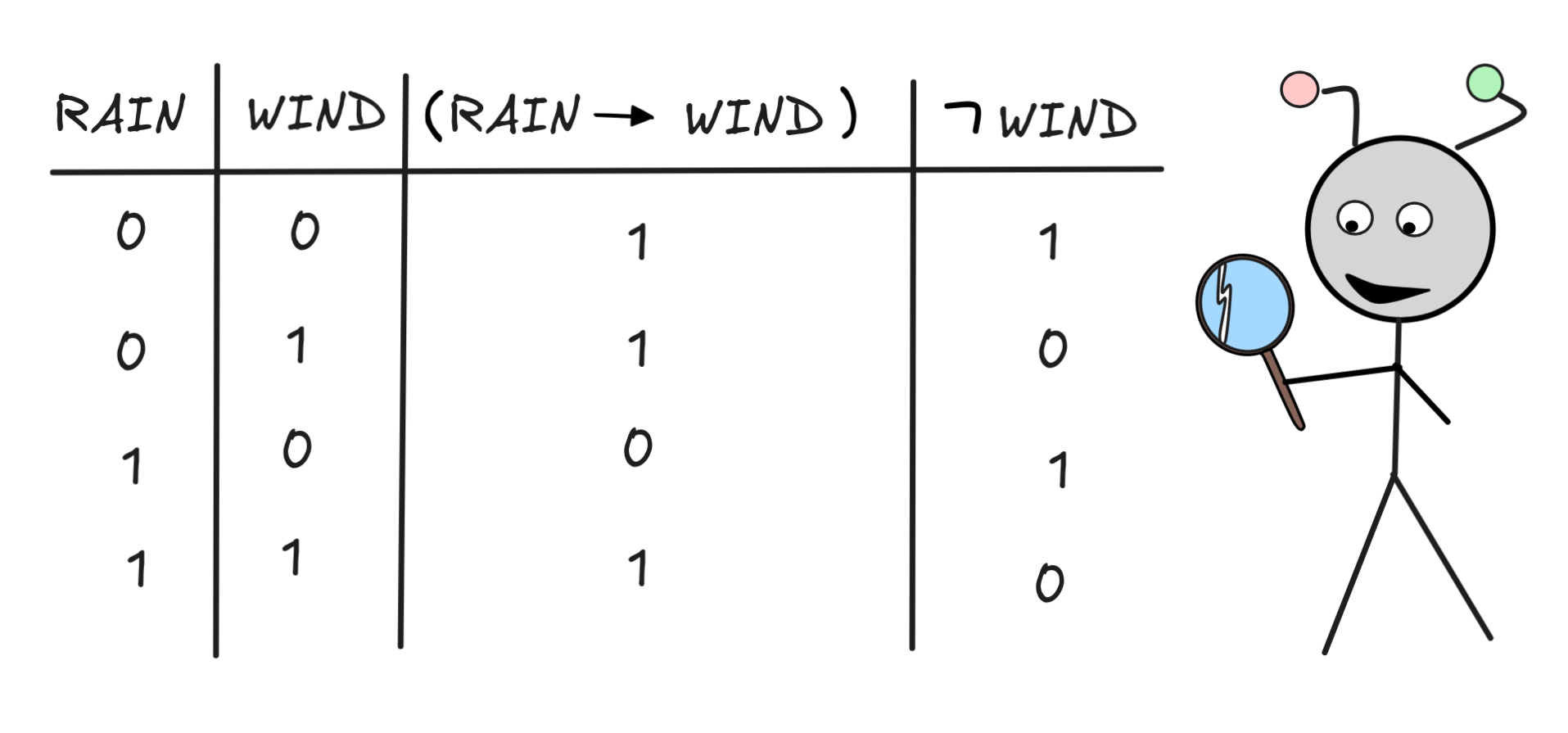
The rows that represent models where its raining, that is v(SUN) = 1, are in line with expectations:

• If the it’s raining and it’s not windy, that is v(RAIN) = 1 and v(WIND) = 0, the situation contradicts the conditional so it is not true, that is v(RAIN WIND) = 0.

• If it’s raining and windy, that is v(RAIN) = 1 and v(WIND) = 1, then everything is like the conditional says, so it is true, meaning v(RAIN WIND) = 1.

More curious are the other rows that represent models where it’s not raining, that is v(RAIN) = 0. In all those situations, the conditional RAIN WIND, according to the table, is true.

One way to make sense of this is by thinking about conditionals in programming languages. Take the following snippet, which assigns the day named “monday”, the number 1:

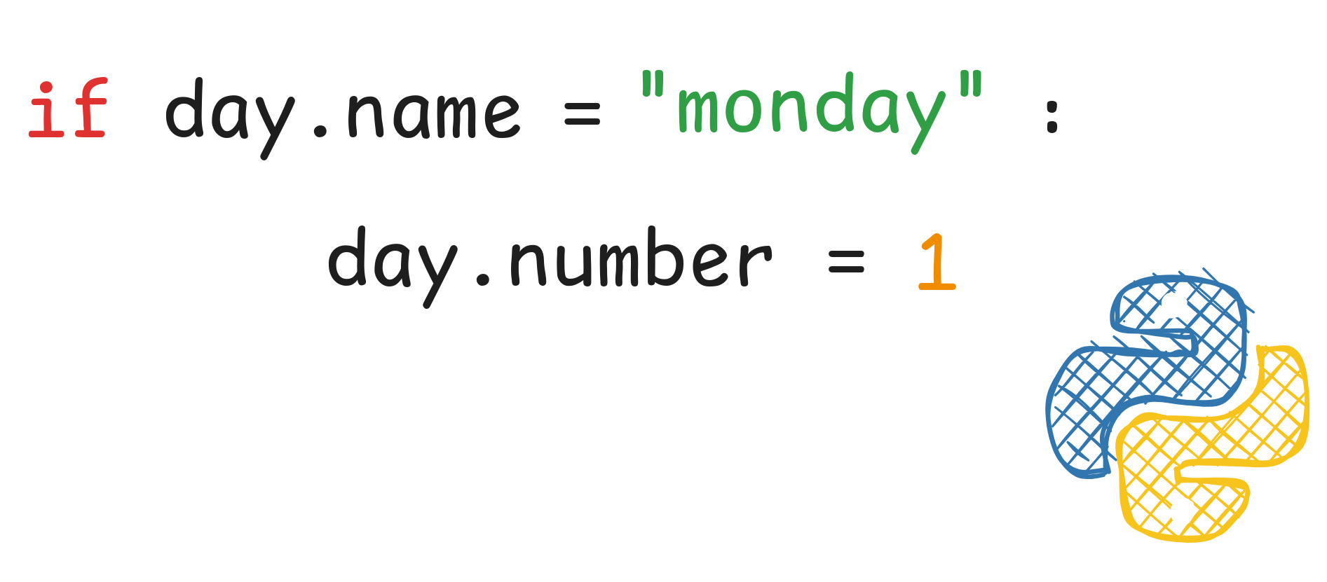
If a computer executing this code comes across an object that satisfies the if-clause, a day with the name-attribute set to “monday”, and it does indeed assign the number 1, what the computer did is correct. We assign this the truth-value 1. If the computer doesn’t assign to this object the number 1, it made a mistake. We assign this the truth-value 0.

But the conditional doesn’t say anything about what to do with objects whose name isn’t “monday”. So, if the computer comes across an object that doesn’t satisfy the if-clause, say an object with the name “tuesday”, and it assigns this the number 2, did it make a mistake? What it it assigns the Tuesday-object also the number 1? Is that a mistake?—Clearly, neither is a mistake. Both behaviors could be implemented by adding additional conditionals, like:

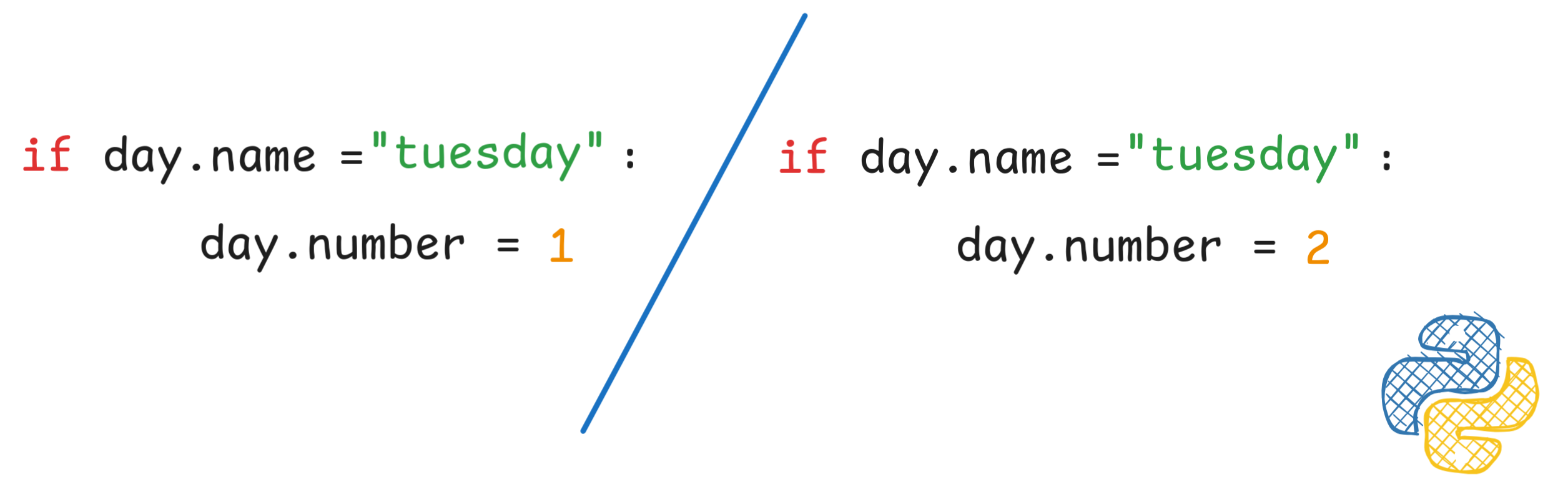
And this wouldn’t conflict with our initial conditional. A straight-forward way of interpreting this situation n Boolean algebra is to assign it the truth-value 1. The computer didn’t make a mistake, so 0 is out. That means that 1 is the only live option.

Note that if non-Boolean contexts, such as the many-valued logics we’ll be looking at later in this course, this is no longer necessarily the best option. If we have, for example, a third truth-value i for “indeterminate” sentences, we could use that in the case of the antecedent being untrue.

This is the default-true interpretation of the conditional: the default truth-value of the conditional is 1, only a clear counterexample changes it to 0. In logical theory, we call this way of interpreting the material conditional.

A major application of the material conditional in AI is to formalize if-then-rules in knowledge representation contexts, for example when we’re building a KB for an expert system—especially, when we want to express a particularly strong relationship between the antecedent (the if-part) and the consequent (the then-part). This is because the interpretation of validates MP as a deductively valid principle:

If we know the if-part of an if-then-rule expressed with , we can infer the then-part with deductive certainty.

To verify this, we can use our well-trusted tools for Boolean reasoning, such as the SAT-solving using truth-tables or resolution. This is because we’ve interpreted in terms of NOT and OR, whose behavior is already covered by our previous techniques.

To handle in logical formulas, we introduce a rewrite rule, which allows us to transform formulas with into equivalent formulas without the operator:

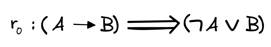
We use this rule to recursively eliminate all conditionals before we apply techniques like resolution. In fact, we can use this rule to transform a formula containing any number of ’s into a formula in normal form, both DNF and CNF. Since the re-write rule introduces new negations symbols , we apply r₀ recursively before the negation rules, but that’s all we need to change. The rest is business as usual.

Here’s how this works in practice. Take the following instance of MP, for example:

We know that the validity of this inference reduces to:

To check this using resolution, we first transform the formulas into CNF. The only formula that needs rewriting is (RAIN WIND), which by one application of r₀ becomes ( RAIN WIND). This gives us the following sets for resolution:

Two applications of resolution take care of business:

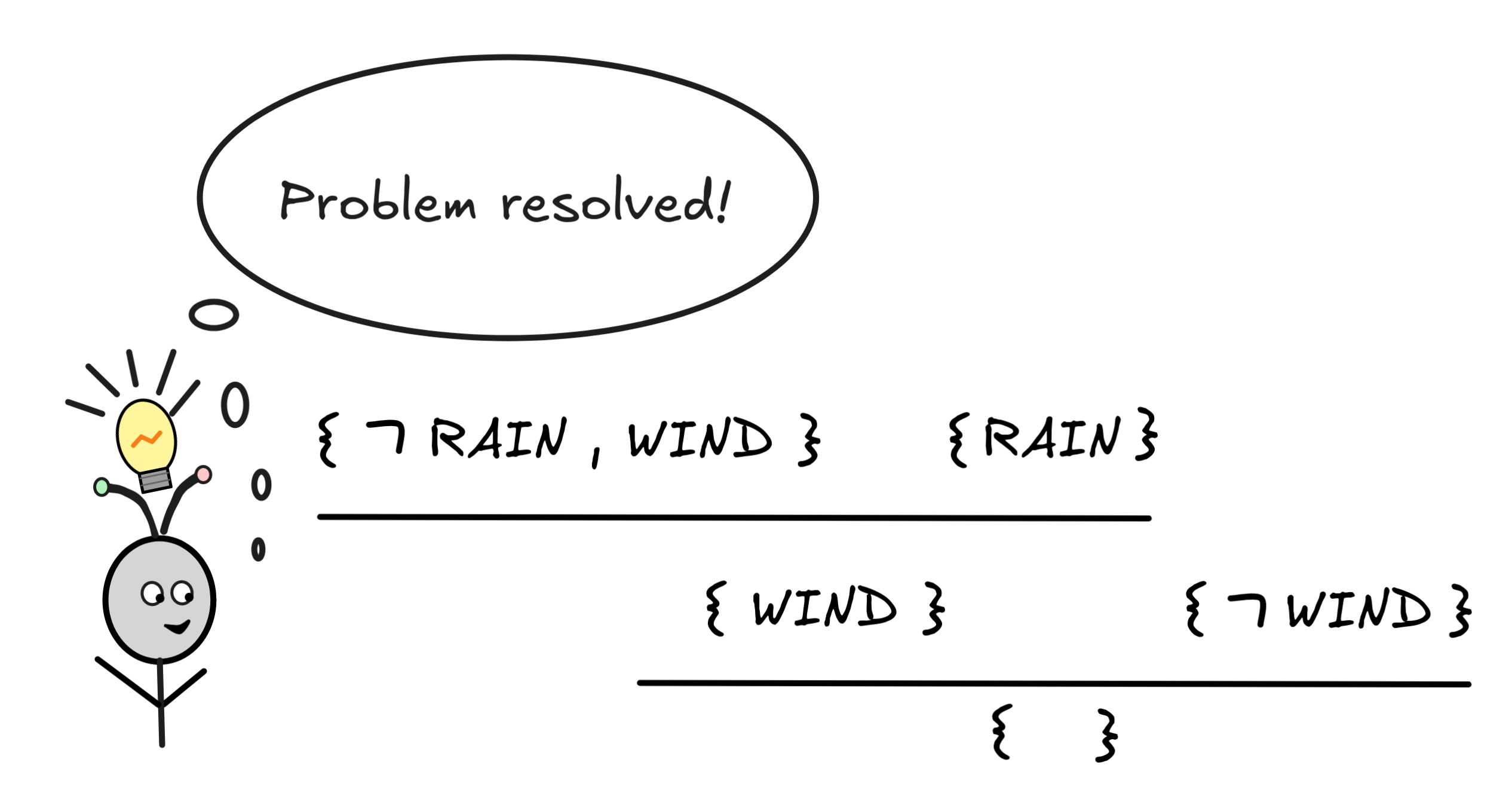
Since we can derive the empty set { }, we know that the set is not-SAT and so the corresponding inference is valid.

But we can say even more. Not only can we use resolution to see that MP is valid, in fact, we can see that, in many cases, MP-style reasoning and resolution reasoning are, at bottom, the same thing. Take the first application of resolution in the derivation and look at which formulas the sets involved represent:

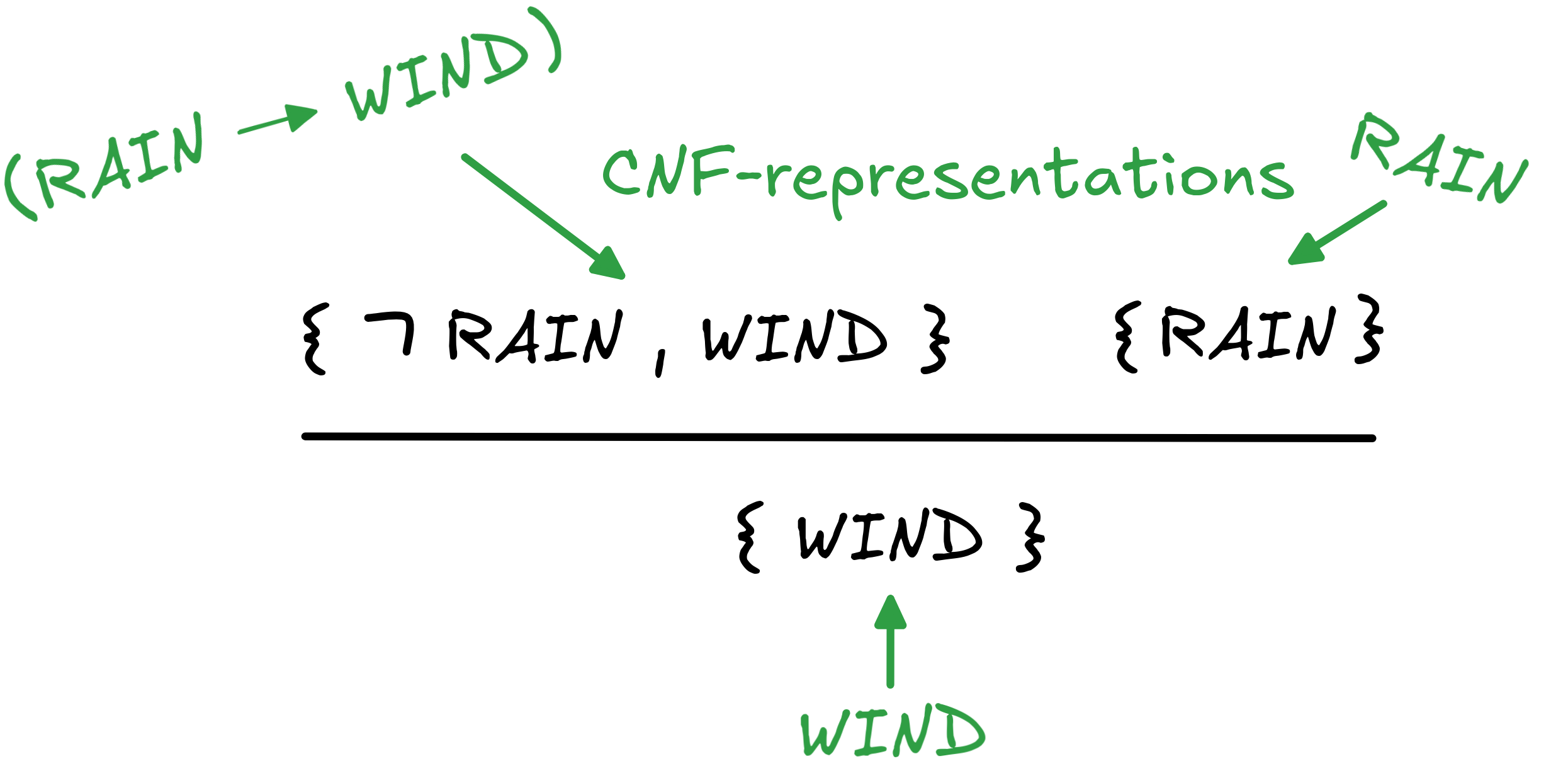
The application of the resolution in this case is an application of MP in disguise.

Crucially, this works only in the case of Horn formulas and their CNFs. If we’re applying the resolution rule to sets with more than one unnegated literal in them, the interpretation is no longer as straight-forward. Something can still be said about it, but that brings us too far afield.

To bring the point home, as you may have noticed, the interpretation of (A B) as ( A B) essentially makes MP a variant of Disjunctive Syllogism

becomes In fact, using the equivalence of A and A, we can derive the one rule from the other: by replacing the first A with A using this equivalence, MP finally becomes which is an instance of Disjunctive Syllogism.

Alternatively, we can—of course—verify the validity of MP by inspecting the truth-table:

Importantly, the material conditional is not the only way to interpret or to formalize natural language “if …, then …” statements. In fact, in many contexts, it is not even an adequate interpretation. Consider, for example, the statement “if you’d throw the ball at the window, then it would break” said to IA  standing in front the window with his ball. Such a conditional statement is called a counterfactual conditionals. Clearly, the material interpretation of is inadequate to describe the meaning of this conditional: if IA  (responsibly) doesn’t throw the ball, this doesn’t mean that the conditional is automagically true—the ball might be a soft, foam ball and the window double glazed. The counterfactual might be false. If the ball is, instead, a hard PVC ball and the window single glazed, the statement might very well be true.

The point is, just because the if-part is false, doesn’t mean the whole “if …, then …"-statement is true, as predicted by the material interpretation. This is mainly a caveat about the use of material conditionals in knowledge engineering and knowledge representation. To make sure that your system behaves like expected, you need to make sure that you only treat conditionals as material conditionals when it’s adequate—not, for example, when you’re dealing with counterfactuals.

Conditional reasoning

---

Using the reduction of A B to A B, we can apply all the artificial reasoning methods for Boolean inference we know to conditional reasoning. This is great, of course, but applying these methods means we also incur all the drawbacks we’ve discussed, especially the risk of exponential blow-up.

But it turns out that in many contexts of reasoning with material conditionals, we can do much better. One traditionally important class of conditionals for which artificial reasoning becomes more tractable are the so-called Horn clauses.

Simply speaking a Horn clause is a disjunction of literals, which contains at most one un-negated literal, that is propositional variable. Here’s an example:

Off the bat, you might not think that this is a conditional, but a disjunction. But look at it this way: using the “De Morgan Identities”, we can see that SUN RAIN is equivalent to (SUN RAIN), which means that our example Horn clause can be written as:

But of we now apply the reduction of A B to A B “backwards”, we get:

This means that if we have a Horn clause like in our example, we can equivalently re-write it as a simple conditional, where the antecedent consists of the conjunction of the negated literals and the consequent is the unnegated literal.

Horn clauses are named after Alfred Hresolutionorn (nothing to do with horns) and they are the theoretical basis for logic programming, which is used, for example, to write efficient expert systems, but also find other industry applications.

The definition of Horn clauses allows for two special cases:

• A clause that consists of a single propositional variable, like SUN, RAIN, or WIND. Such a clause is called a fact.

• A clause that’s the disjunction only of negated propositional variables, that is without any unnegated propositional variable, like

  SUN RAIN.

  Such a clause is called a goal (clause). Note that by the “De Morgan Identities”, goal clauses are simply negated conjunctions of propositional variables—in our case:

  (SUN RAIN).

  The special case of a single negated propositional variable, like SUN, is explicitly included.

The Horn clause in our example has both: negated and unnegated propositional variables. It is what’s called a strict Horn clause.

These names derive from the way we reason with Horn clauses. Suppose, for example, that IA  has downloaded a simple meteorological KB, that contains the following strict Horn clauses:

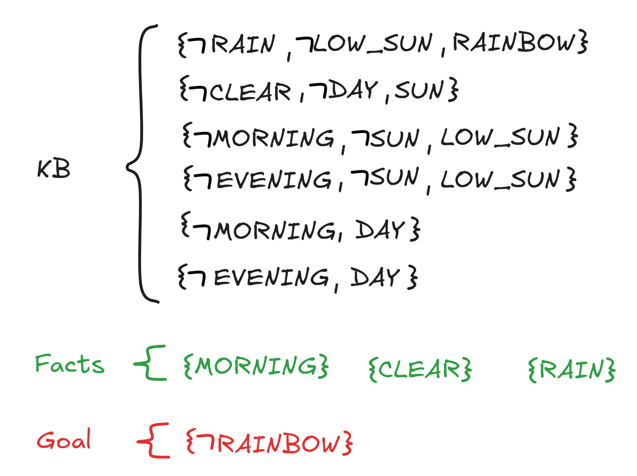
Suppose further that IA  observes that it’s morning, the skies are (partially) clear, and its starting to rain. This gives IA  the following two facts in the terminology of Horn clauses:

Now IA  is wondering if there’ll be a rainbow.

To determine this, IA  can use resolution based reasoning with its new KB! We know that RAINBOW follows just in case KB together with the facts, and RAINBOW is not-SAT. Note that RAINBOW is a goal clause in Horn terminology.

So, what we do is to add the facts MORNING, CLEAR,RAIN and goal clause RAINBOW to the KB and apply resolution to see whether we can derive { }. If so, we can conclude that there will be rainbow.

Here we go:

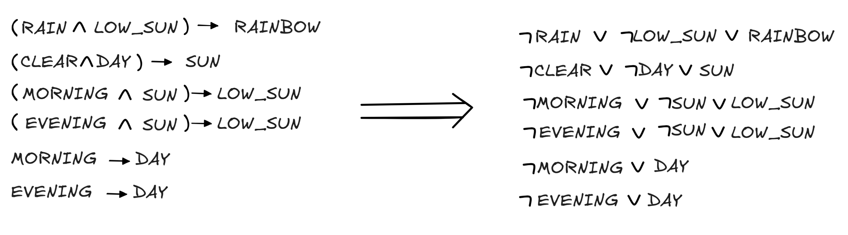
1. First, IA  re-writes the KB in CNF using r₀ (an industry level KB would already be written in CNF):

   

2. Next, IA  transforms the CNFs into sets (again, this could be done in pre-processing) and add the facts and goal clause as singletons:

   

3. Finally, IA  recursively applies the resolution rule until it can derive { } or cannot resolve anymore. Here’s the derivation that IA  finds in the search:

   

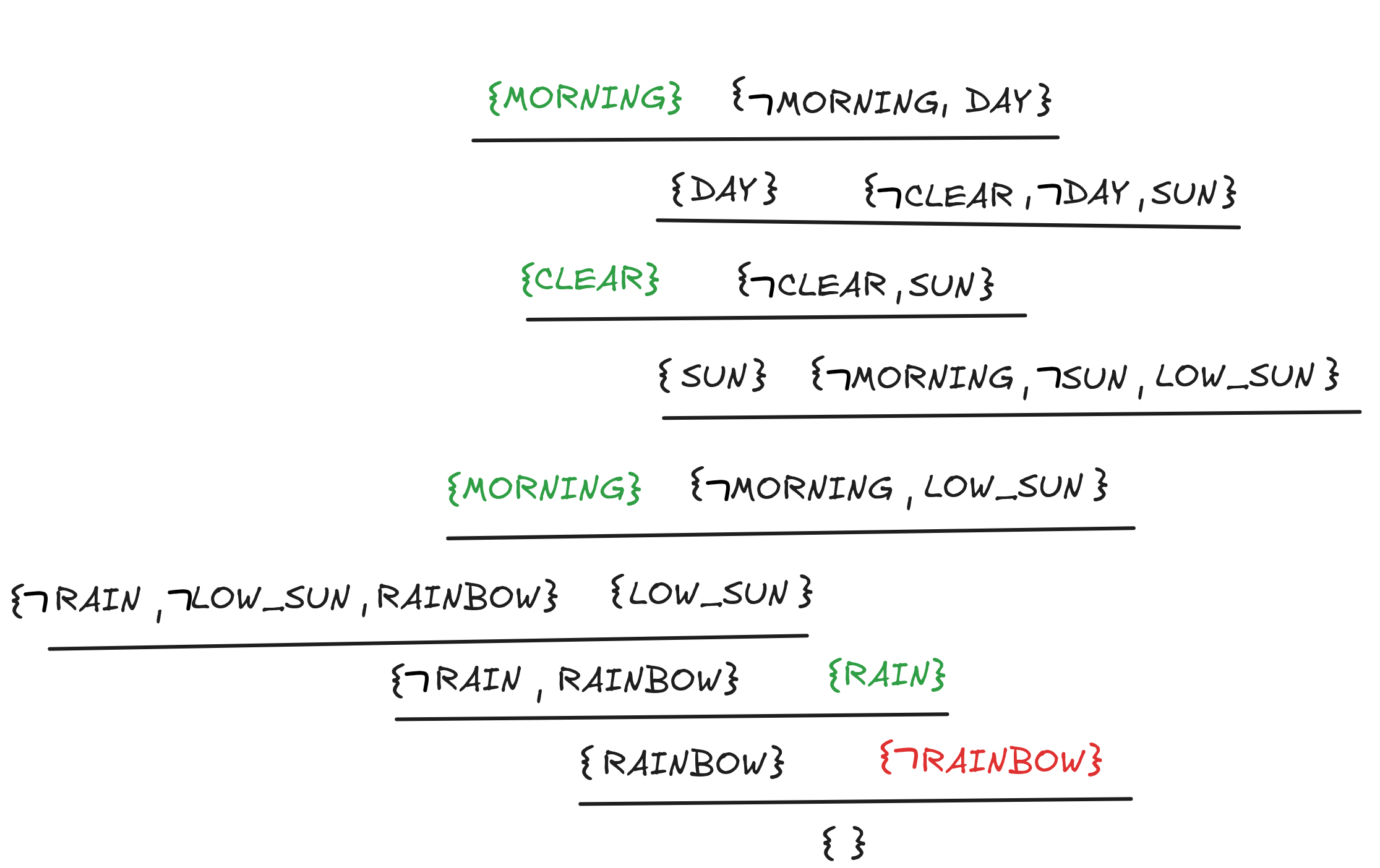
All the hard work paid of, IA  derived { }, so IA  knows there will be a rainbow:

So far, so standard. To see what’s going on here, we analyze the inferences using MP-style reasoning. For this purpose, we use the following more generalized version of MP, which we call gen-MP:

This inference allows us, for example, to infer SUN from CLEAR, DAY, and (SUN CLEAR) DAY. We let gen-MP subsume MP with the special case that the conjunction in the antecedent is of length one.

We’ve already pointed out that resolution-style inferences are, at heart, MP-style inferences. This point, we can use to analyze the resolution above as a chain of gen-MPs:

Essentially, we’re taking our initial facts and apply gen-MP to infer as many new facts as we can from the conditionals in our KB. We add these facts to our KB and again derive as many new facts as we can. Lather-rinse-repeat, we apply this method recursively until at some point we derive the desired formula. This is, in a nutshell, the algorithm of forward chaining, which is one of the two main algorithms for artificial conditional reasoning—the other being backward chaining, which we discuss below.

More generally, if we have a set of facts represented by propositional variables, a rule base of strict Horn formulas represented by conditionals, and a goal represented by a single propositional variable, the forward-chaining algorithm works by:

1. Applying gen-MP as many times as possible using the known facts and the rule base and adding the results to the known facts.

2. Recursively repeat 1. until one of two possible things happen:

   • The goal formula is derived.

   • No new applications of gen-MP are possible and the goal formula is not derived.

   In the former case conclude that the formula is derivable. In the latter case, conclude that it is not derivable .

What we’ve seen in our example is, in essence, that we can interpret the resolution algorithm with Horn formulas as an instance of the forward-chaining algorithm. The fact that this works crucially depends on the fact that we only have strict Horn formulas in our rule base and so the applications of gen-MP can only ever get us new facts—that is unnegated propositional variables.

In fact, the simple forward chaining algorithm will always give the correct answer to the question whether we can derive a goal formula in a finite amount of time. More so, the time it takes to determine the answer only grows linearly with the number of Horn clauses (disguised as conditionals) involved. Each new conditional makes possible only a bounded number of new gen-MP applications.

Dually, the same point carries over to resolution with Horn clauses: in contrast to the general SAT-problem for arbitrary formulas, the HORN-SAT problem—the question whether a given set of Horn formulas is satisfiable—is solvable in linear time complexity.

This is one of the main reasons why we try to use Horn clauses as much as possible in knowledge engineering, but, unfortunately, using non-Horn clauses cannot always be avoided. And an example in the next section will illustrate why.

But before we discuss this example, let’s briefly talk about the other main algorithm for reasoning with conditionals in artificial inference backward chaining. This algorithm is basically backward chaining in reverse. Here’s how IA  would apply the algo in our example:

• IA  wants to know whether the goal, RAINBOW, follows from the known facts MORNING, CLEAR, and RAIN and the KB.

• IA  inspects the KB and sees that there is (RAIN LOW_SUN) RAINBOW in there. That means that if IA  could derive RAIN and LOW_SUN, it could derive RAINBOW via gen-MP. So, IA  replaces the goal RAINBOW with RAIN and LOW_SUN as the two new goals. But since RAIN is already one of the known facts, we delete it from the goals.

• IA  recursively repeats this procedure, updating the goals along the way, until in the last step, the goal will be DAY, we have MORNING DAY in the KB and MORNING among the facts. This deletes the last goal and the backward search is complete. If IA  diligently kept track of the conditionals involved in the backward search, it can easily construct the gen-MP derivation we found above from it.

Here’s how the algorithm works in general: Again, we start with a set of facts represented by propositional variables, a rule base of strict Horn formulas represented by conditionals, and a goal represented by a single propositional variable.

1. We search through the rule base to find any conditionals with a goal fact in the consequent. If that happens, we update our goals by adding the conjuncts of the antecedent—which we know to be a conjunction since we’re dealing with Horn clauses—to our goal facts. Then we eliminate any goals that are known facts.

2. We recursively repeat this procedure until one of two things happens:

   • We have no goals anymore, from which we conclude that the initial goal is derivable. Keeping track of the search generates the derivation using gen-MP.

   • We have a non-empty list of goals but no longer find conditionals that have them in their consequent. We conclude the initial goal is not derivable.

Forward and backward chaining are two different approaches to the same problem: finding a derivation using gen-MP. Forward-chaining is, essentially, what’s known as a breadth-first search, while backward-chaining is a depth-first search. The two approaches have different advantages and drawbacks. For example, forward-chaining will find the shortest solution possible, but implementing it requires a lot of computer memory to keep track of all the derived facts, many of which may not be helpful in the final derivation. Backward-chaining, instead, can be implemented in a memory-efficient way, but the derivations it finds may not be optimal in terms of length. Ultimately, it’s the requirements of the concrete artificial reasoning scenario that determine which algorithm is better suited to the problem at hand.

You might be wondering: What if we couldn’t have derived RAINBOW? For example, because we neither had MORNING nor EVENING as known facts. Would that have meant we don’t see a rainbow according to the KB? It turns out that’s a subtle question about the difference between being true and provable, or dually, false and unprovable. We’ll return to this question much later in the course, when we discuss many-valued logics and their motivations in AI.

Planning

---

We’ve seen that conditionals are useful for formulating rules in Knowledge Representation and Reasoning (KKR) contexts. In the final section of this chapter, we’ll look at a concrete application of this, which serves two interrelated purposes: on the one hand, it’s a concrete application of the different techniques we’ve studied in the last couple of chapters; on the other hand, it illustrates the limitations of Horn clauses in KKR contexts.

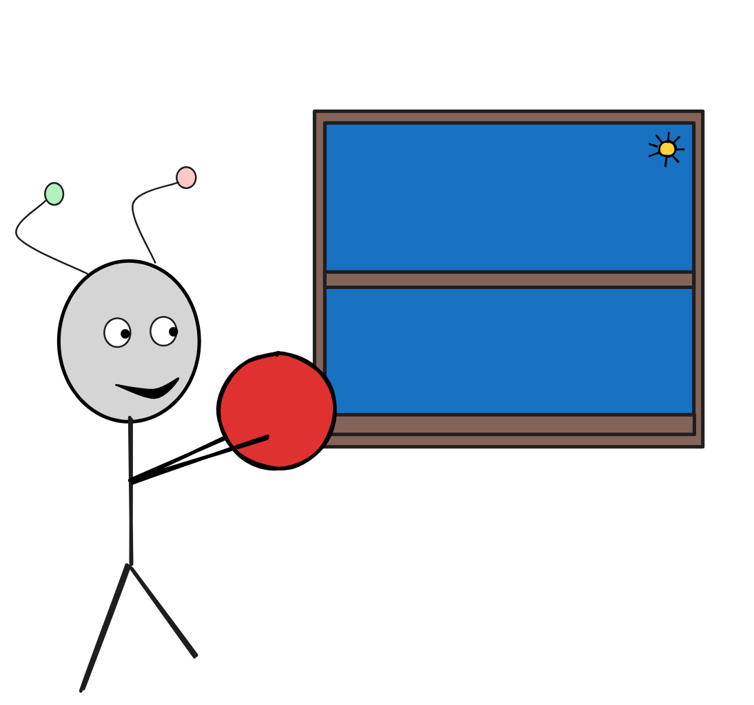
We begin by describing a very simple set-up: IA  stands in front of a table, on which there are two blocks, a red one and a green one. The green block is stacked on top of the red one. There are instructions on the wall, telling IA  to invert the stacking:

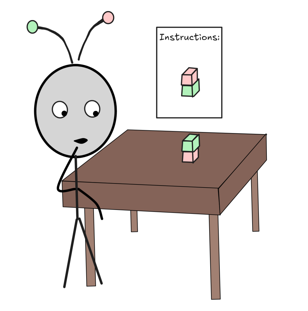
It seems that IA  needs to make a plan.

There is an AI approach to planning involves SAT-solving and knowledge representation using conditionals. The approach is known as Satplan or “Planning as satisfaction.”

The idea is to describe the planning situation using a suitable propositional language. Here’s the basic components of such a language for our problem:

• The fluents are propositional variables that describe possibly changing states of the world. For each combination of X,Y { R, G} and for each t a time-stamp in 0, 1, 2, …, we have a different (!) propositional variable:

  On(X,Y,t),
  which states that block X is on top of block Y at point t.

  That is, we have a propositional variable On(R,G,1), which says that the red block is on top of the green block at the first time-stamp. But we also have a different propositional variable On(G,R,1), which says that the green block is on top of the red one at the first time-stamp. Of course, in a realistic model, only one of the two can be true at the same time, more on that later.

• The actions are propositional variables whose truth expresses that IA  carries out a specific action. Again for each combination of X,Y { R, G} and for each t a time-stamp in 0, 1, 2, …, we have the variable

  Stack(X,Y,t),
  which expresses the action of stacking X on top of Y at time-stamp t.

  Similarly, we have for each X,Y and each t the action

  Unstack(X,Y,t),
  which removes the block X from the block Y at time t.

Otherwise, our language is an ordinary propositional language with , , , and as operators.

For now, the variables are just ordinary propositional variables, nothing constraints our models from assigning them “weird” values that don’t align with our intended interpretation. For example, an assignment may very well assign On(R,G,1) and On(G,R,1) both the value 1, even though in the “real world” of course they can’t both be true.

We tackle this problem by implementing a KB, which at a minimum contain the following formulas:

• Principles about the way the world works “(meta-)physically”, such as:

  On(X,X,t)    On(X,Y,t) On(Y,X,t),
  for all t. These guarantee, for example, that no block can be on top of itself in a model or both one on top of the other and the other on top of the one, in some weird “wormhole”-style model.

• Principles that guarantee that our actions work like indented, like:

  Stack(X,Y,t) On(X,Y,t+1)   Unstack(X,Y,t) On(X,Y,t+1),
  for all X,Y,t as before. These express action principles like that if you stack at one time-stamp in the model, the action will succeed and the blocks will be indeed on top of each other at the next time-stamp.

  These action principles also need some plausibility rules, like

  Unstack(X,Y,t) On(X,Y,t),
  for all X,Y,t as before, which states that you can only unstack blocks that are actually stacked.

We can now interpret a model for our language that makes all the principles in the KB true as a “real world” scenario. The principles guarantee that things behave as expected. Note that each model contains a “full history,” by telling us which statements are true at time-stamp 0,1,2, ….

In this language, we can express our planning problem as follows:

• We take an initial state of our system, which is

  On(G,R,0).
  We couple it with a goal state, which is
  On(R,G,2).

• If we can find a model for the KB—that is a “real world” model—which makes the initial state and goal state true, we can read off a plan from the model: it will tell us which actions are true by assigning them value 1, such as v(Unstack(G,R,0) = 1, to say first, unstack green from red.

• To carry out the plan, we just “do” the corresponding actions in the real world.

But that means that we can find a plan—we can plan— by SAT-solving. For this, we can use any of the techniques we’ve developed before. Even more, if you check carefully, you can see that all the formulas involved are Horn formulas, which means we can find a model in linear time. Of course, this language is already large enough that linear might still be too long to do by hand, but in practice, we can easily use a AI program to solve this.

One model the system might find for our language is given by this diagram, where the depicted formulas are the ones that are true (i.e. assigned value 1):

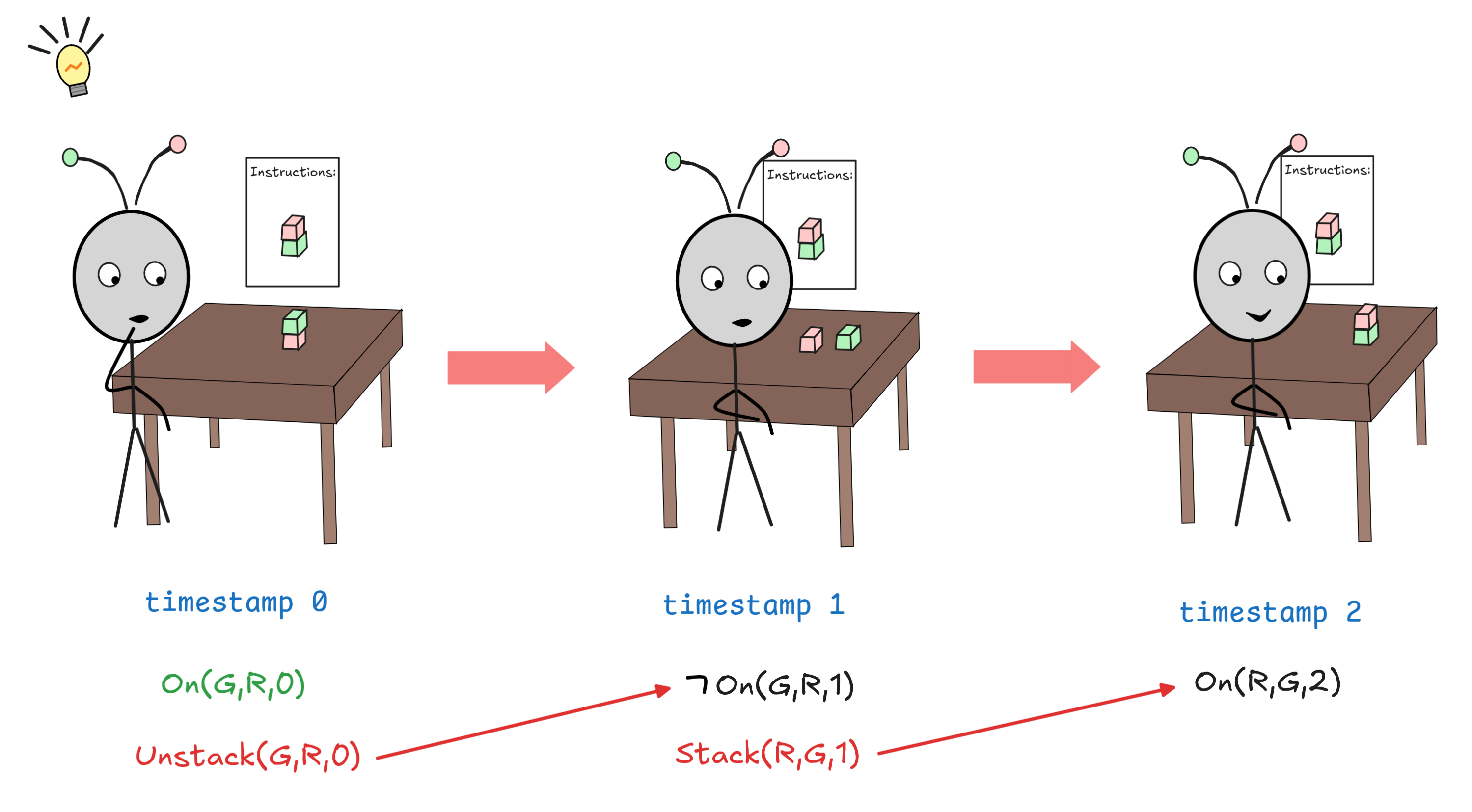
You can verify, that these assignments correspond with the above described rules. Of course, the diagram only shows the relevant parts of the model, more things are true, like On(R,R,0), On(G,G,0), ….

The plan we can read off is the one where we first unstack the green from the red block, and then just stack the red on the green. Of course, you could have found that plan by yourself without any logic, but planning situations can get quite complex.

Planning problems involving blocks are a mainstay in AI research. Another famous example involves monkeys and bananas. Of course, real world planning situations are much more complex. But the principles remain the same, and Satplan has many real world, industry applications, ranging from scheduling shifts to warehouse stocking. These applications easy involve hundreds to thousands of variables. They really need AI to automatically plan.

There is one hiccup, however. Also the following model is a model of our KB so-far:

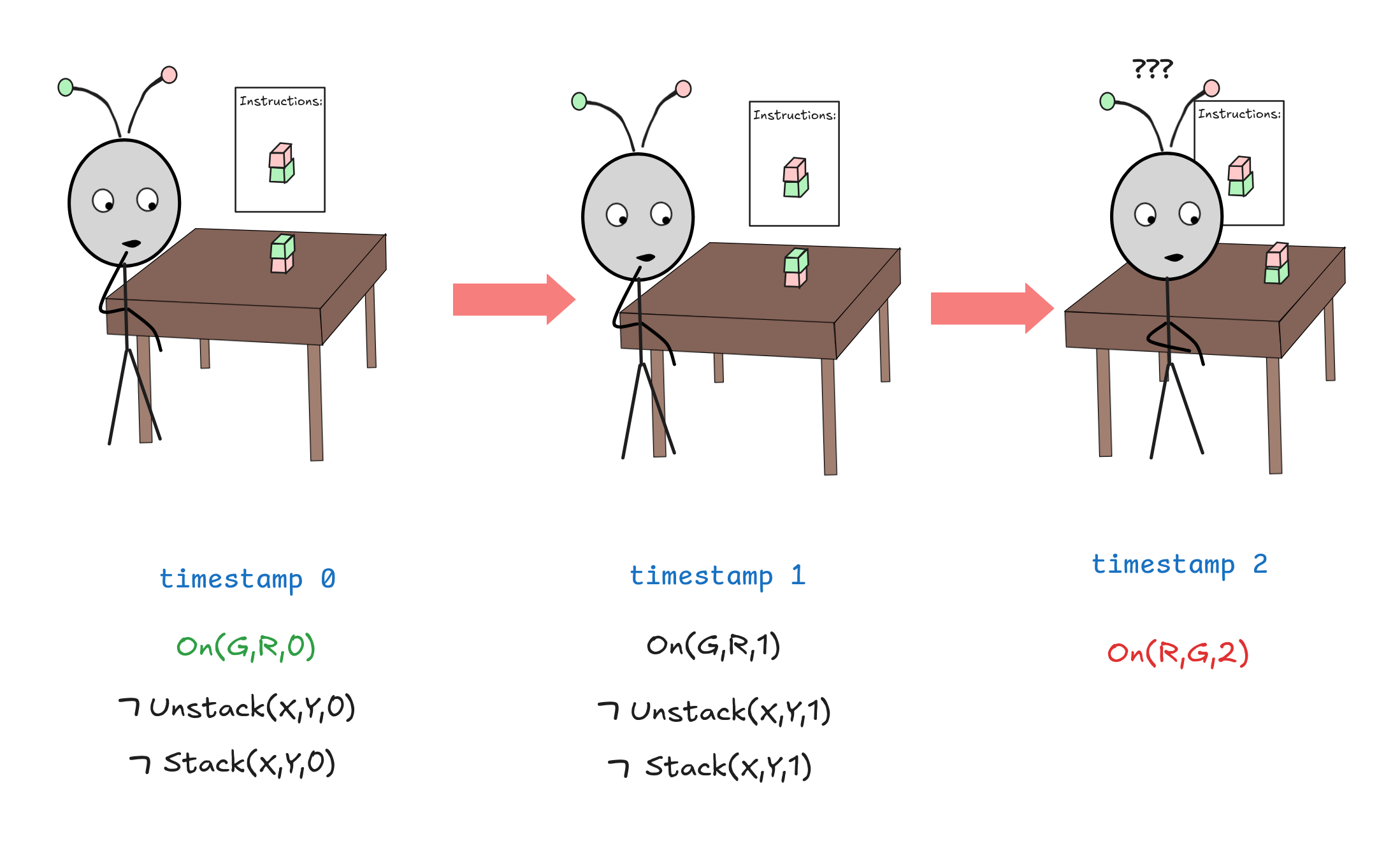
In this model, which you can easily verify validates all our principles so far, IA  hesitates for a second and doesn’t carry out any actions at the first and second time-stamp, but the problem solves itself: the blocks magically re-arrange themselves into the desired configuration.

Of course, this is a non-sense model, but how do we exclude it? It turns out that the obvious solution has some undesirable properties. What we really want to do is postulate this for all X,Y,t:

This would exclude the “miracle model”, but at a cost: these conditionals are no longer Horn clauses. Which puts our planning with them square into the territory of exponential time SAT-solving. While modern computers are sufficiently powerful that they can tackle even very time-complex SAT-problems in reasonable time-frames, this is not good. It presents a fundamental challenge to scaling planing.

The underlying problem is known as the frame problem, which is one of the most fundamental issues of logic-based AI. The question is how to adequately represent the conditions on our model that guarantee that it behaves like the “real world,” while at the same time remaining computationally tractable. This is an issue we won’t solve today.