FOL Inference

It turns out that automating inference in FOL is a hard problem.

Take our standard inference, for example:

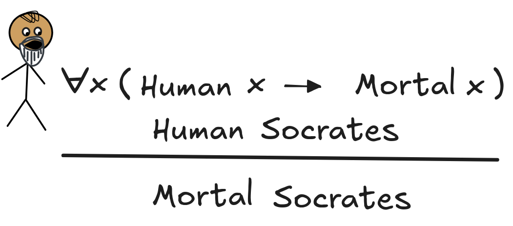
It’s actually rather straight-forward to see that this inference is deductively valid in FOL. Suppose, we’ve got a model, M, where both premises are true, that is:

• M x (Human x Mortal x)
• M Human Socrates

If we unfold the former using the truth-conditions in models, we get:

• For all d D, M Human d Mortal d.

But Socrates D. Since Socrates is a name for Socrates —by definition—we know that:

• M Human Socrates Mortal Socrates

But the second premise was that M Human Socrates. So by simple Boolean reasoning—essentially just MP—we know that:

• M Mortal Socrates.

For this line of reasoning, we didn’t need to think about what our domain looks like, what the extensions of Socrates, Human, and Mortal are. What we’ve seen is that regardless of all these things: the truth of the premises in any FOL model is sufficient for the truth of the conclusion. In other words, the inference is deductively valid:

x (Human x Mortal x), Human Socrates Mortal Socrates

The relative ease with which we showed the inference’s validity might spark the hope for a relatively straight-forward theory of mechanized FOL inference. We’ve developed a series of inference techniques for Boolean and propositional reasoning, such as truth-tables, SAT-solving, and natural deduction. We might hope, at this point, that they just carry over to FOL modulo some adjustments for the more complicated syntax and semantics.

But appearances are deceiving. First, note that we needed to think in a very human way through the truth-conditions to see that the inference is valid. For example, we realized that the denotation of Socrates lives in our domain, and therefore satisfies the open formula Human x Mortal x. But how could a machine do that? Or, put differently, how can we algorithmically check for the validity of an FOL inference?

This is where the trouble begins. In propositional logic, we could just brute force search through all the models of the premises using the truth-tables. But this doesn’t work in FOL. While in propositional logic, all that mattered for the truth of a formula is which of its propositional variables are true, in FOL, we need to know more: which objects there are, what the terms denote, and what the properties express. But that means that not only do we need to search through all distributions of truth-values over the atoms, we need to search through all through possible domains and interpretations of vocabularies across them.

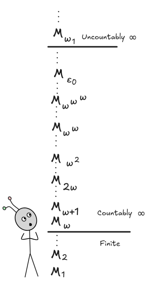
But there are many possible domains. Every set of objects could be the domain of a model. And the universe of sets is … enormous to put it mildly. At the very least, it’s infinite, so we simply can’t search through it in finite time complexity.

That rules out brute force, but perhaps there could be some smart algorithm, some effective method that solves the problem for us, that can figure out for any given FOL inference, in a finite amount of time whether the inference is valid.—It turns out that the answer is: there can’t be!

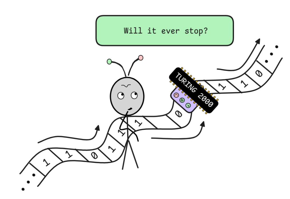This is a consequence of Church and Turing’s answer to the halting problem. Without going into too much detail, Curry and Turing independently showed that there can’t be a single algorithm that determines in a finite amount of time whether any given computer program “halts”—meaning it doesn’t get stuck in an “ infinite loop”. The model of computation that they used in this proof—the lambda calculus in Church’s case and Turing machines in Turing’s case—is so general in nature that it encompasses any reasonable form of AI algorithm we can think of. The details of the proof are out of scope for us, but roughly the idea is that we can reduce the halting problem to a validity problem in FOL. This proof is one of the great intellectual achievements of the twentieth century and one of the ways in which research in pure logical theory is highly relevant to current AI-research: we know that we shouldn’t even try to fully automate FOL inference.

What we can do is to deal with the consequences: we can tackle the question what, given that we can’t fully automate FOL inference, we can still achieve. And it turns out that there’s quite something. AI research has yielded a toolbox of techniques for FOL reasoning, partially and fully automated, theorem proving and checking. These tools are the basis for many recent advances in domain-specific reasoning.

At the end of this chapter, you will be able to:

• use the method of unification to find applications of FOL inference rules to quantified FOL formulas

• transform FOL formulas into CNF and apply the resolution method to search for countermodels

• use natural deduction rules for the quantifiers to find logical proofs in FOL

• verify such proofs in Lean

Unification

Let’s begin by looking at our example inference again:

x (Human x Mortal x), Human Socrates Mortal Socrates

We’ve seen that the inference is valid using semantic reasoning, but now we’ll investigate how to show this using inference rules.

The aim is to apply something like MP to obtain the desired result. The idea is to focus on the reasoning that if x (Human x Mortal x) is true, then Human x Mortal x is true for all values of x. So if we set the value of x to the denotation of Socrates, we can use this to infer that Human Socrates Mortal Socrates is true. Then, since Human Socrates is true, we can use MP to infer that Mortal Socrates is true as well.

To cash this out, we need to think about how to reason with universally quantified variables, like the x in this case. The powerful idea we’ll be developing throughout this chapter is that we can drop the quantifier   and reason with the open formula

Human x Mortal x

(Human x Mortal x), Human Socrates Mortal Socrates

What remains to be done is to find a mechanizable way of determining that we should set the value of x to Socrates. The way this works, formally, is using the method of unification.

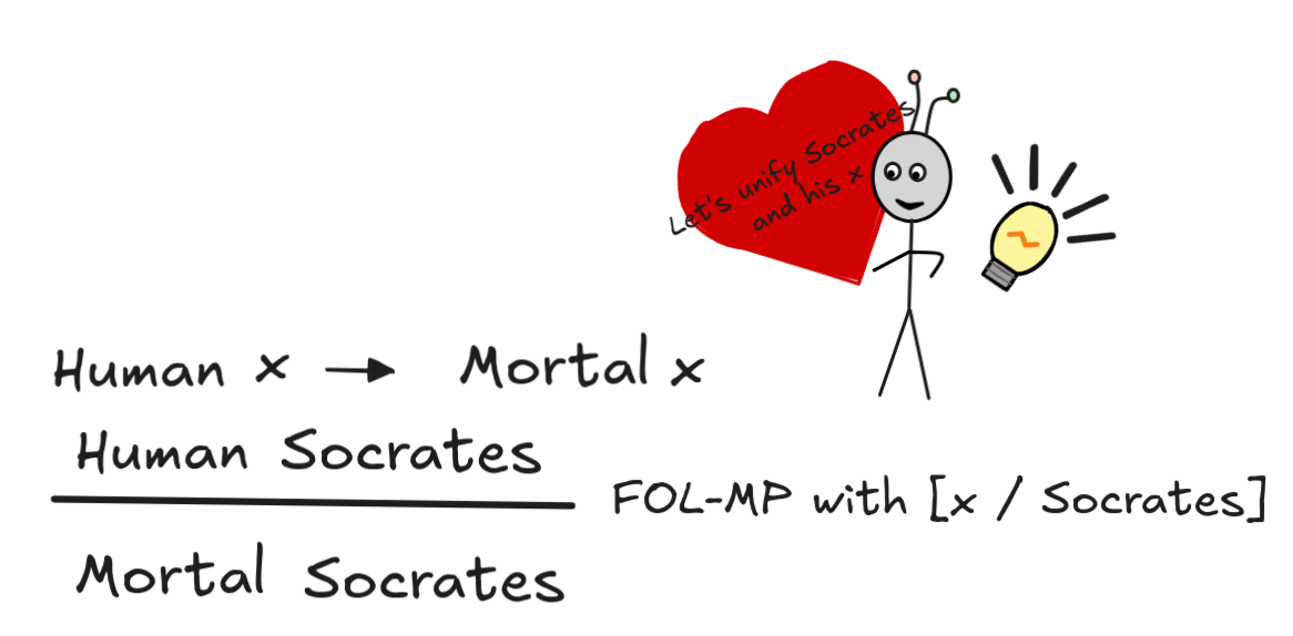
What we need to do in order to be able to apply MP, what we need to do is to set the value of x in such a way that the Human x in Human x Mortal x becomes Human Socrates. The obvious way of doing this is to replace the x with the constant Socrates to obtain Human Socrates Mortal Socrates. Formally, this happens with the operation of term substitution, which we looked at in the syntax of FOL. That is the substitution [x / Socrates] gives us:

(Human x Mortal x)[x / Socrates] = Human Socrates Mortal Socrates

where our premise Human Socrates is syntactically identical to—not only equivalent, but literally identical to—the antecedent of the conditional. A substitution that has this property is called a unifier of the two formulas with the unification partners [Human Socrates, Human x].

That is, we can understand our inference as an instance of a special MP variant for FOL:

That is, FOL allows us to infer the consequent of an open conditional with free variable x from a sentence if there is a unifier which makes the antecedent of the conditional and the sentence syntactically identical.

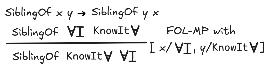
It’s rather straight-forward to generalize this rule to antecedents with multiple variables in the premise and antecedent. Take the following deductively valid inference, for example:

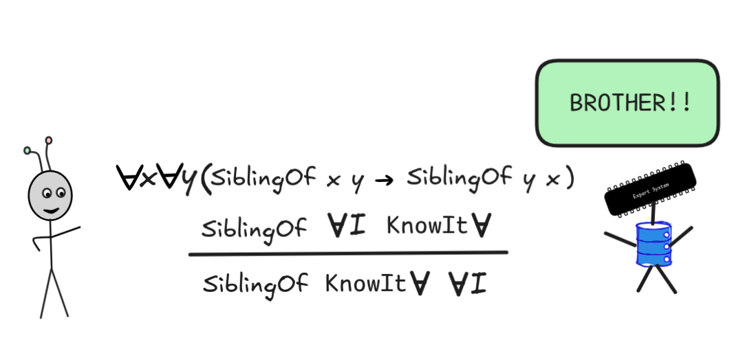
To apply the method we’ve just described, we’d simply drop both universals and use the unifier

[x / I, y / KnowIt  ]

This gives us a first shot at FOL inference: we can generalize MP to inferences with universally quantified conditionals using unification. It turns out that unification is an extremely powerful method for automated inference. It is, for example, also the method that underpins how Lean figures out “under the hood” which disjunction you wanted to use in an application of Or.inl, for example.

Remember that the natural deduction inference from A to A B using Intro corresponds to the lean apply Or.inl h, where h : A is a proof of A. Note that you don’t need to tell Lean here that you’re other disjunct is supposed to be B. If you later want to apply MP-style reasoning with some premise g : (A ∨ B) → C to obtain a proof of C, you do this with code like this:

1
2

apply g 
apply Or.inl h

Lean figures out that the other disjunct in your application of Or.inl must have been B using unification. Under the hood, when you apply the rule, it infers a proof of A X for a meta-variable X. Then, when you tell it to apply the proof of the conditional (A ∨ B) → C, lean uses a unification algorithm to infer that if X is B, the application is valid, and so it applies the unification and continues. This is just one of the ways, in which unification-based algorithms make our lives a little bit easier in artificial inference. It also allows us to use the backward chaining and forward chaining algorithms when our KB contains suitable conditionals.

In practice, there are different algorithms for efficiently search for unifiers for two first-order terms. The most basic one, due to Robinson, you will explore in the exercises. Importantly, the unifiability of two terms is a decidable problem: we can correctly tell with a single algorithm in finitely many steps whether any two terms can be unified or not.

But just like with propositional chaining, there are limitations to this method. In propositional logic, we looked at conditionals with disjunctive antecedents as an example, like in the inference:

((RAIN WIND) COLD)  (COLD HEATING)  RAIN

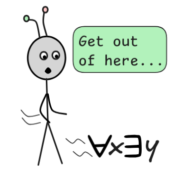
In FOL, we also have , so we have these kinds of inferences, but there are also problems with quantifiers in conditionals. Consider the following inference, for example:

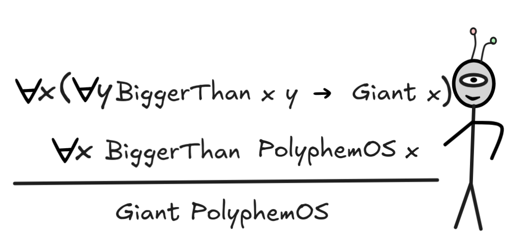
This inference is straight-forwardly seen to be valid: If it’s true that anyone bigger than everyone is a giant, and PolyphemOS is bigger than everybody, then PolyphemOS is a giant. In fact, applying our strategy of dropping all the universals , we might think we could do the following:

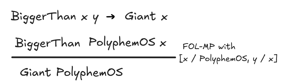
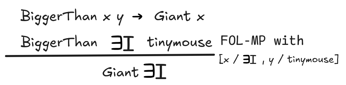
This looks like a logical proof of the validity of the inference, but actually something went wrong. To see this, consider the following inference:

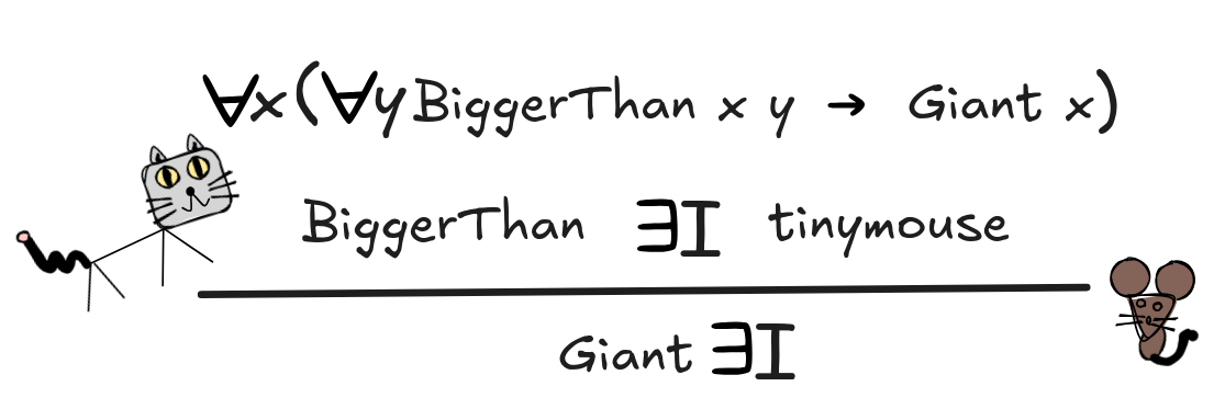
This inference is clearly deductively invalid: Even if it’s true that anyone bigger than everyone is a giant, the fact that IE   is bigger than tinymouse doesn’t mean that IE  is a giant. It’s rather simple to find a formal FOL countermodel to the inference.

But if we could just drop all universals like we just did for the inference involving PolyphemOS, the following would seem to show that the inference is valid:

What went wrong here is that the y was nested in the conditional antecedent and doesn’t really work like a “real” universal. To see this, we transform the premise using the equivalence of A B and A B, which also holds in FOL:

• x ( y BiggerThan x y Giant x) is equivalent to x( x Bigger Than x y Giant x).

That is, the premise says that everything is either not bigger than everything or a giant. In fact, we can use the following FOL equivalence to transform this even further:

• y BiggerThan x y is equivalent to y BiggerThan xy

To say that x is not bigger than everything is to say that there’s something that x is not bigger than. Using this equivalence:

• x( x Bigger Than x y Giant x), and thus x ( y BiggerThan x y Giant x), is equivalent to x( y Bigger Than x y Giant x).

Either there exists something that x is not bigger than, or x is a giant.

Writing the premise in this form explains why the simple unification-based FOL-MP cannot be applied here, since there’s an existential is involved. To handle such more general inferences, we need to move to a more powerful system.

FOL Resolution

While there is no brute force, truth-table-style method for FOL, we can use resolution to check for satisfiability and thus consequence—although there are some caveats.

Note that once we’ve defined the notion of a model and truth in a model for FOL, we get the same relation between deductively valid inference and satisfiability that we had in propositional logic:

P₁, P₂, … C   if and only if   not SAT{P₁, P₂, …, C }

Here, P₁, P₂, …, C can be any FOL formulas and the notion of a set being satisfiable (or SAT) is simply that there’s a model, in which all the formulas are true.—FOL resolution is a method for checking for SAT in this sense.

So, just like in propositional logic, we can check for satisfiability to check whether an inference is valid. And that’s what FOL resolution does. The only caveat here is that while in propositional logic, resolution is a decision procedure—that is, it correctly tells us in finitely many steps whether a set is satisfiable/an inference is valid—in FOL, the method is “only” sound and complete: if we can derive an empty sequent or contradiction from a set using resolution, we know its unsatisfiable, and for each unsatisfiable set there is such a derivation. But crucially, as a consequence of Church and Turing’s theorem, there is no algorithm that in general is guaranteed to find the this derivation—even if it exists. We still need to be “smart” about it. This puts a damper on the ambition of fully automating FOL reasoning, but it also presents an opportunity to develop smart algorithms that perform imitate human-level skills—or even achieve superhuman abilities—at finding FOL derivations.

So, here’s how FOL resolution works. In the simplest cases, we’ve actually already seen resolution at work in the FOL-MP with modus ponens: just like in propositional logic, the simplest applications of resolution are just cases of MP. The first step for implementing this involves re-writing. If we take our inferences involving Socrates, after dropping the universal, we can transform the conditional into a disjunction using the well-established equivalence between A B and A B. We get:

Human x Mortal x

The other premise and negation are already of the right form:

Human Socrates   Mortal Socrates

With these transformations in place, we can move to sets like in the propositional case and apply resolution rules to derive the empty set { }:

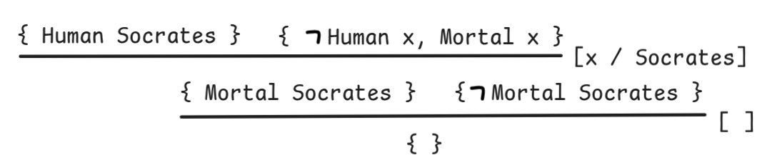
The idea here is that we can resolve on two formulas just in case the can be unified using a substitution such that the one becomes the negation of the other. Here, we resolve on Human Socrates and Human x using the substitution [x/Socrates]. This substitution needs to be applied to all the remaining formulas in the two sets that we’re resolving, which is why we retain Mortal Socrates from (Mortal x)[x/Socrates]. Sometimes, there is no substantial unification necessary, since the formulas are already resolved, as in the last inference. The formulas we’re eliminating in the resolution is also called the pivot of the application.

For the general form of resolution, we need to talk about CNFs for FOL. Remember that the resolution system assumes that all formulas are in CNF, which means that they are conjunctions of disjunctions of literals. To carry this notion over to FOL, we just need to adjust the notion of a literal. In propositional logic, a literal is a propositional vairable or its negation. In FOL, it’s simply an atomic formula or its negation. That is

Human x, x = Socrates, BiggerThan Socrates fatherOf(y), …

There is also a corresponding notion of a DNF, which in AI and automated inference is not as important as the CNF. This is mainly because there is no truth-table style method for SAT-solving in FOL, which is one of the main things that DNF’s are good for in propositional logic. So, we’ll focus on CNFs.

Just like in propositional logic, there’s an re-write algorithm for transforming any formula into CNF. Crucially, this transformation doesn’t give us an equivalent formula, but an equi-satisfiable formula, meaning that the CNF is satisfiable if and only if the original formula is. The reason why we don’t get full equivalence has to do with quantifiers.

Note that CNFs are, by definition, free of quantifiers. This means, we need when we transform a formula into CNF, we need to eliminate the quantifiers—and this cannot, in general, be done in such a way as to preserve strict equivalence. But we can preserve satisfiability, which is all we need for our SAT-based approach.

Enough theory, let’s look at how this works in practice. The algorithm is a recursive re-writing with rules, just like before. In fact, all the re-write rules from the propositional algorithm are also rules in FOL, we just add to them. To remind ourselves, here’s how the rewriting works in propositional logic:

1. We recursively rewrite all conditionals into disjunctions using:

   r₀: A B A B

2. We recursively push all negations inward using:

   r₁: A A
   r₂: (A B) A B
   r₃: (A B) A B

3. We recursively transform disjunctions of conjunctions into conjunctions of disjunctions using:

   r₄: A (B C) (A B) (A C)
   r₄': (A B) C (A C) (B C)

To handle the quantifiers, we need to add new re-write rules. We discuss them in turn. The conditional re-writing step, 1., stays the same. For the second step, we add two quantifier rules:

2. We recursively push negations inward using r₁—r₃ plus:

   r₆: x A x A
   r₇: x A x A

Now, before we can go on, we need to make sure that there cannot be any confusion about quantifier binding. Remember that formulas like the following are valid FOL expressions:

x (Human x x(Human x Mortal x))

That is, different quantifiers can use the same variable. This can lead to confusion when we drop quantifiers and needs to be avoided. The solution is to re-formulate all formulas (equivalently) in such a way that each quantifier occurrence in the formula uses a unique variable. So, for example, instead of the previous formula, we write:

x (Human x y(Human y Mortal y))

This sort of variable renaming is called α-renaming and happens in its own step. In order to implement this, we first create two stack of pairwise distinct variables

In practice, we just need for every quantifier occurrence in the formula a separate variable, but for simplicity, we just assume that there’s an infinite stack. We use the operation called pop to remove the first element from the stack and return it. That is, pop [x₁, x₂, x₃, …] returns x₁ and leaves the stack as [x₂, x₃, …]. Using this machinery, we implement the following re-write step:

3. We recursively re-name the variables using:

   r₈: x A α A[x / α], where α = pop varx
   r₉: x A α A[x / α], where α = pop vary

That is, if at some point we come across a quantifier expression, we replace the variable quantified over with the first variable from our stack and replace all free occurrences of the variable originally quantified over with that variable as well.

This re-write step gives us, for example:

x (Human x x(Human x Mortal x)) y₁ (Human y₁ x₁(Human x₁ Mortal x₁))

If there are more variables involved, the variable naming get’s more complex, but every quantifier get’s its own variable:

x( Human x y ( z(ParentOf x z ParentOf y z))) …

… …

x₁( Human x₁ y₁ ( x₂(ParentOf x₁ x₂ ParentOf y₁ x₂)))

There is a small complication, when we apply this step in resolution SAT-solving. We need the variables to be unique not only within a formula, as in our example, but also across formulas. That is, when we have in our set x Human x and x Mortal x as separate formulas, we need to transform them into something like x₁ Human x₁ and x₂ Mortal x₂ (results may vary depending on how many other variables occur in other formulas “in between”).

We solve this by applying the entire algorithm to all formulas in our simultaneously, moving through the steps in unison and then sharing the variable stack across the different formulas. The use of pop prevents us from ever using the same variable twice in the transformation.

So far, all our transformations where equivalent transformations in the sense that the formula that comes out the other end is deductively equivalent to the original formula—it always has the same truth-value in all models. This changes in the next step, where we eliminate the quantifiers.

The process for eliminating universals xᵢ will be simple: we’ll just drop them. But first, we have to deal with the existentials using a procedure known as Skolemization, after the logician Thoralf Skolem. This procedure is rather complex and in practice, you’ll typically “play it by ear” and not apply the recursive algorithm we’ll describe now. At the same time, it’s important to understand how the algorithm works to understand what happens in resolution-based SAT-solvers for FOL.

To illustrate the idea, let’s take our formula from earlier:

x ( y BiggerThan x y Giant x)

After running through the transformation steps up to α-renaming, we arrive at the formula:

x₁( x₂ Bigger Than x₁ x₂ Giant x₁)

What this formula says is that for each x₁ either there exists an x₂ which x₁ is not bigger than or, otherwise, x₁ is a giant. We want to re-write this fact—if not equivalently, at least equi-satisfiably—without without using existential quantifiers. The crucial insight of Skolem’s that makes this possible is that all we need to do is to pick some object for each x₁. That is, dependent on any value for x₁, we need to get an object that behaves according to the formula. In mathematical terms, this means that there’s a function, which picks for every value of x₁ such an object. This function, we can represent using a so-called Skolem-function, which we shall write (in this case) as skolem¹. That is, we can write the formula as:

x₁( Bigger Than x₁ skolem(x₁) Giant x₁)

While this formula is not equivalent to our original formula, it is equi-satisfiable—there exists a model where the one is true iff there is one where the other is. And if we now drop the universal quantifier, we’re left with a completely quantifier free formula:

Bigger Than x₁ skolem(x₁) Giant x₁

This is the formula we can use for FOL resolution.

But in the more general case, a few things can happen that we need to discuss. First, when there’s more than one existential quantifier in a formula, then we need have different skolem-functions for each of them to guarantee equi-satisfiability. Take the following, for example:

x₁( y₁ BrotherOf x₁ y₁ y₂ SisterOf x₁ y₂)

This formula says that everybody either has a brother or a sister. After Skolemization, the formula becomes:

x₁(SiblingOf x₁ skolem₁ x₁ y₂ SisterOf x₁ skolem₂ x₁)

The use of different skolem-functions is necessary since if we’d use the same function, we’d get:

x₁(SiblingOf x₁ skolem x₁ y₂ SisterOf x₁ skolem x₁)

This would make the brother and sister the same person, since—obviously—skolem x₁ = skolem x₁.

And then, there’s dependence on more than one universally quantified variable:

x₁ x₂ y₁ CommonAncestor x₁ x₂ y₁

Every two people have a common ancestor. The Skolemization of this formula is:

x₁ x₂ CommonAncestor x₁ x₂ (skolem x₁ x₂)

Note: The parentheses are added for readability only.

We can now describe the general re-write rule of Skolemization. Watch out, this will be rather complex. As I said, in practice, you mostly won’t work through the complex algorithm but transform directly. We assume that for each arity n, we have a list of Skolem functions:

In the case where n = 0, we call them Skolem constants and treat them as such.

Further, for the purpose of the recursion, we need to keep track of the universally quantified variables that an existential depends on. We denote the list of these variables (in order) by deps. That is, in

x₁( x₂ FriendOf x₁ x₂ x₃ y₁ CommonEnemyOf x₁₃ x₃ y₁)

y₁

Note that if deps = [ ], then we use Skolem constants. For example,

y₁ Human y₁ y₂ Human y₂ Human skolem⁰₁ Human skolem⁰₂

4. We recursively Skolemize the existential quantifiers using:

r₁₀: yᵢ A A[ yᵢ / skolemᵢdeps]

As we said, this re-write rule is rather complex, in practice relatively straight-forward to work out.

Now that we’ve eliminated the existentials, we can drop all the universal:

5. We recursively drop the universal quantifiers using:

r₁₁: xᵢ A A

In the very last step, we distribute if necessary:

6. We recursively transform disjunctions of conjunctions into conjunctions of disjunctions using:

   r₄: A (B C) (A B) (A C)
   r₄': (A B) C (A C) (B C)

Applying rules 1—6 of this algorithm simultaneously for all formulas in a set, yields a set of CNF formulas. These we can transform into sets of clauses and like before and start apply resolution.

Take, for example, in our inference about PolyphemOS:

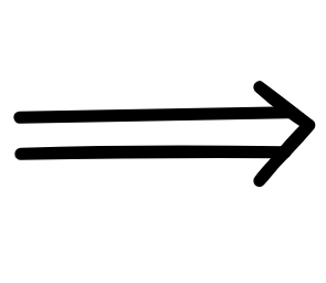
x( y BiggerThan x y Giant x), x BiggerThan PolyphemOS x Giant PolyphemOS

In order to check this inference for validity, we check the following set for satisfiability using FOL-resolution:

{ x( y BiggerThan x y Giant x), x BiggerThan PolyphemOS x, Giant PolyphemOS }

We get the following CNF formulas:

BiggerThan x₁ skolem x₁ Giant x₁

Giant PolyphemOS

Using FOL-resolution, we derive the empty sequent in two steps:

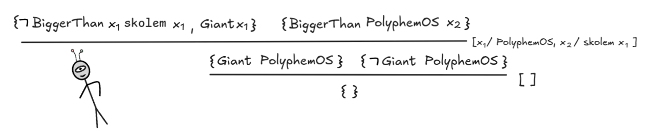
If, instead, the second premise would have been BiggerThan IE tinymouse, we’d have ended up with:

BiggerThan x₁ skolem x₁ Giant x₁

Giant IE

And the resolution algorithm would have stopped after one application:

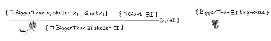
Thus, we can prove that the inference is invalid, as desired.

To conclude the discussion, here’s how FOL resolution can be formalized as a general FOL inference rule:

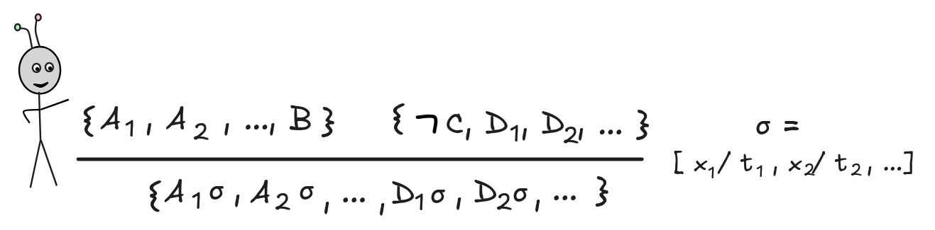
Here σ = [ x₁ / t₁ , x₂ / t₂ , …] is a substitution, which unifies B and C, that is:

These are the basics of FOL resolution. Before we conclude our discussion, it’s worth remarking that FOL resolution is a sound and complete proof system for FOL. That is, there is a derivation of the empty sequent from the CNFs of the premises and the CNF of the negation of the conclusion if and only the inference is valid. But in contrast to propositional logic, the system is not a decision procedure: we cannot fully automate it as an algorithm and trust that it will return the correct answer—valid or invalid—for any given inference. Let’s try to understand what can go wrong.

The problem is with inferences where the countermodel is necessarily infinite. Take the following FOL formulas written in infix notation using the binary predicate ≤, for example:

1. x y x ≤ y
2. x (x ≤ x)
3. x y z((x ≤ y y ≤ z) x ≤ z)

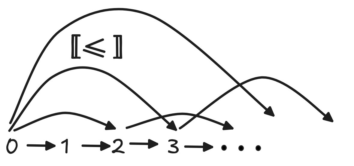
If you think about what a model of these formulas looks like, you notice that it must contain an infinite sequence of objects, which successively get bigger and bigger. The following is a graph-representation of such a model, where the domain consists of the natural numbers {0, 1, 2, …} and ≤ is simply the “real” smaller than relation on the

numbers:

Now, add any statement to 1.—3. that doesn’t follow from them. For example, 1 ≤ 0. It really doesn’t matter what this statement is, since if we apply the resolution algorithm to the set containing 1., 2., 3., and Prime 3, it will never terminate. To see this, let’s first transform the statements into CNF set form. We get:

{ (1 ≤ 0) }

{ x₁ ≤ (skolem x₁) }   { ( x₂ ≤ x₂) }

{ (x₃ ≤ x₄), ( x₄ ≤ x₅), x₃ ≤ x₅ }

Now suppose we implement our algorithm such that it always first tries to resolve on { x₁ ≤ (skolem x₁) } and it begins with { (x₃ ≤ x₄), ( x₄ ≤ x₅), x₃ ≤ x₅ }. The following happens:

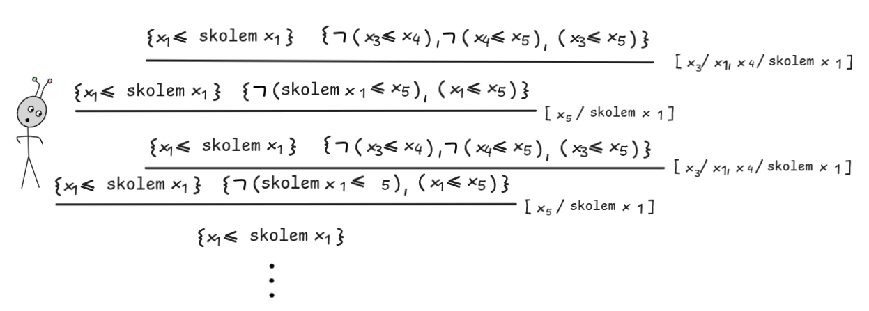
We got stuck in an infinite loop, which means the algorithm never terminates and we never get the answer that the conclusion doesn’t follow. This doesn’t mean that it does follow, we can easily construct a countermodel, such as the one we’ve just described above. But the algorithm doesn’t find it. Of course, with our superior human-intelligence™️, we can see that this loop will occur and try to avoid it, but the bottom line of the Church-Turing theorem is that we can’t find a systematic, algorithmic way of excluding such loops.

As you can see, the resolution algorithm gets quite involved and complex, even at the general, example-driven level of description we’ve used here. This is why it’s best left to computers. There are various industry-level implementations, with various optimizations, which perform well at the tasks involved—much better than humans could. For example, the method of validity checking we’ve just described is the basis for Prover9, which is oftern used as a benchmark for FOL automated theorem provers.

Natural deduction and Lean

While FOL resolution is useful for computer implementations, it’s not the most straight-forward to work with when trying to write logical proofs for in a human-readable way. For this, we need to look to natural deduction. There are also sound and complete Hilbert calculi, sequent calculi, and tableaux systems for FOL, but natural deduction is the system that most closely resembles human-style inference. As such, it is the system that is most frequently used in AI applications, such as proof verification in mathematics or the more recent advances in artificial mathematical reasoning using hybrid LLM-proof assistant systems.

The natural deduction system for FOL extends the system for propositional logic with four new rules:

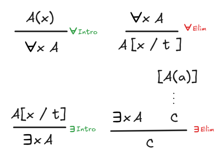
Each of these rules has some special side-conditions, which require some explanation. Let’s discuss them in turn.

The first rule,  Intro, has the side-condition that the variable x may not occur free in any undischarged assumption the we’ve used to derive A(x). The idea is that if we can derive A(x) without making any assumptions about x, this means that the argument holds for any x. Here’s an example of the rule at work:

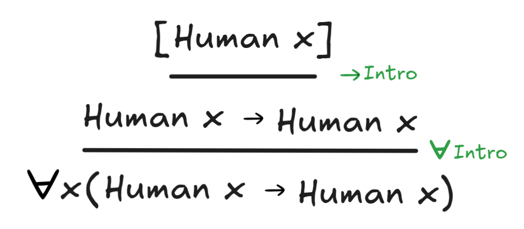
This is a rather trivial inference, but it illustrates the idea well. We can show that if x is human, then x is human without any open assumptions left using Intro. Since this proof doesn’t assume anything about x, we conclude that it holds for all x. Every human is human is a logical truth, we can proof without any undischarged assumptions.

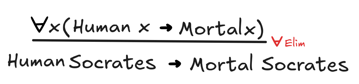
For a slightly more interesting application, we first need to talk about Elim. This rule is perhaps the most straight-forward one: it allows us to infer from a universal statement that holds for all x, that it holds for any specific object, designated by any term t. For example, it gives us the inference:

There is a side-condition with this rule as well: we can use any term t as long as it is not bound after the substitution. This blocks, for example, the following invalid inference from being an instance of Elim:

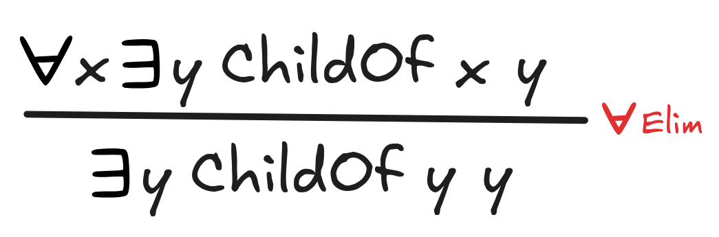
From everyone being the child of someone, it doesn’t follow that someone is their own child. The side-condition blocks this invalid rule application.

In combination, Intro and Elim can be used to prove some more interesting logical laws of FOL, such as the following:

x(Black x White x) x Black x x White x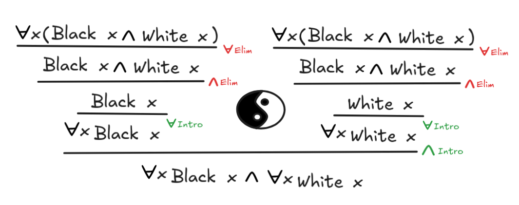

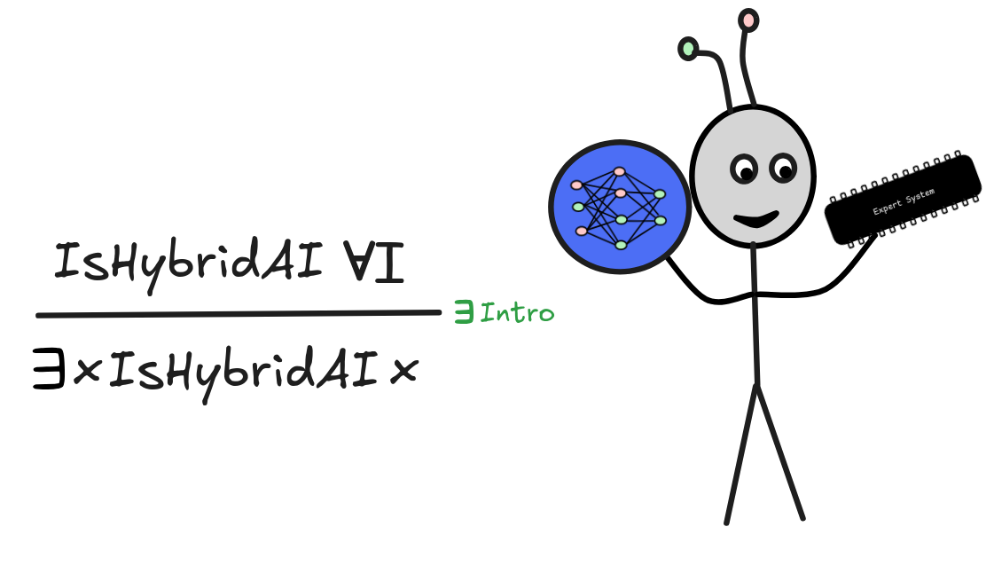
The rule  Intro is also relatively straight-forward: it allows us to infer that there exists an object satisfying a property from any concrete object instantiating that property. For example, we have:

There are no side-conditions for this rule. There are conditions for the Elim rule. This rule captures the idea that what we can infer from an existential claim is what we can infer from some arbitrary instance of the existential. All we know is that some object satisfies the property. If from this assumption, without assuming anything else about that object, we can derive a conclusion, we can infer that conclusion from the existential. This idea is captured in the side-condition that the constant c in the assumption, may not be used anywhere else in the derivation.

Here’s a valid inference using the rule:

x Black x x (Black x White x)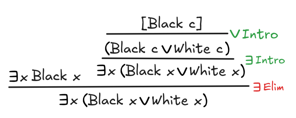

If there’s a black object, then there’s an object that is black or white—namely that unspecified object that is black.

The introduction and elimination rules for and are together sound and complete for FOL: Gödel’s completeness theorem entails that for every deductively valid inference there exists a corresponding natural deduction derivation and vice versa. Of course, there cannot be a sure-fire way of finding such a derivation as this would contradict the Church-Turing theorem.

To conclude our discussion of FOL—and classical deductive logic in general—let’s look at how we can verify FOL inference in Lean. The Curry-Howard Correspondence, which we’ve taken as the starting point for our ventures into proof verification in propositional logic, extends in a natural way to FOL.

Remember that in propositional logic, we used the type Prop to model propositions that are true or false in Lean. In FOL, we need to extend this setting with terms and predicates that we apply to them. For this purpose, we introduce a new kind of type, the Term-type, which contains all the objects that we talk about. A (unary) predicate, then, can be understood as a function from terms to propositions, formally an object of the type Term → Prop. The idea is if we apply a predicate, like Human, to a term, like Socrates, then we obtain a proposition, namely Human Socrates. Here is how we’d declare Black and White as unary predicates in Lean.

1

 variable ( Term : Type ) (Black White : Term → Prop)

Just like for each intro and elim rule of natural deduction there was a corresponding pair of Lean rules, we have Lean rules for the introduction and elimination rules for the quantifiers.

Let’s begin with Intro. Essentially, Lean treats the universal quantifier just like the existential: what we need to show is that from the assumption of an arbitrary x, we can derive a proof the proposition in question—then we can conclude that the property holds for all x. Here’s the Lean proof that corresponds to our simple inference which shows that all humans are human:

1
2
3
4
5
6

variable ( Term : Type ) (Human : Term → Prop)

example : ∀ x, Human x → Human x := by
  intro x
  intro human_x
  exact human_x

Click this link to run this code in your browser.

That is, Lean treats a proof of a universally quantified statement as a kind of conditional: if x is an arbitrary object, then x is human if it is human.

Correspondingly, the rule of Elim corresponds application: to infer an instance from a universal quantifier, we take

Here, for example, is the Lean verification of our inference:

x(Human x Mortal x) Human Socrates Mortal Socrates

1
2
3
4

variable ( Term : Type ) (Human Mortal : Term → Prop)

example (Socrates : Term) (h : ∀ x, Human x → Mortal x) : Human Socrates → Mortal Socrates:= by
  apply h

Click this link to run this code in your browser.

Our more complex proof of everything’s black and everything’s white from everything’s black and white is verified like this:

 1
 2
 3
 4
 5
 6
 7
 8
 9
10

variable ( Term : Type ) (Black White : Term → Prop)

example (h : ∀ x, Black x ∧ White x ) : (∀ x, Black x) ∧ (∀ x, White x) := by
  apply And.intro
  · intro x
    apply And.left 
    exact h x
  · intro x
    apply And.right 
    exact h x

Click this link to run this code in your browser.

Finally, for the existential quantifier, we have the tactics Exists.intro and Exists.elim. The tactic Exists.elim takes as arguments a proof of a disjunction and a proof of a conclusion from the assumption that an arbitrary object (which needs to be intro‘ed) has the property in question. Exists.elim just requires a proof of an instance.

Here’s how they work in action in our combined inference to show that if there’s a black thing, there’s a black or white thing:

1
2
3
4
5
6
7

variable ( Term : Type ) (Black White : Term → Prop)

example (h : ∃ x, Black x) : ∃x, Black x ∨ White x := by
  apply Exists.elim h
  · intro c black_c
    apply Exists.intro
    apply Or.inl black_c

Click this link to run this code in your browser.

There is, of course, much more to know about the use of classical deductive logic in AI and its verification, but we’ll leave it at that. Next, we turn to different realms—namely non-classical logic.