By: Johannes Korbmacher
Logic-based learning
In this, rather short chapter, you’ll learn about how we handle learning on a logic-based approach to AI.
We’ll discuss two approaches:
-
a deductive logic-based approach, known as belief revision, and
-
an inductive, probability-based approach, known as Bayesian updating.
Both approaches find applications in AI, even though Bayesian updating is by far more popular. In the end, though, symbolic learning methods are not the gold standard for machine learning—statistics is. In this chapter, we’ll see why.
We’ll only touch the surface of the broad field of symbolic learning in this chapter, but at the end, you’ll have an idea of the basic approaches and challenges they face.
Belief revision
We start with the deductive approach: belief revision. Suppose we have knowledge base \mathsf{KB}, which contains our knowledge about the relevant subject matter. For belief revision, it’s important that we understand our \mathsf{KB} as a set of formulas, meaning \mathsf{KB}\subseteq \mathcal{L}. In addition, we assume that we’ve already explored all the logical consequences of our \mathsf{KB} and added them to the base so that it satisfies the following closure condition:
- If \mathsf{KB}\vDash A, then A\in KB
Another way of expressing this condition is to say that our \mathsf{KB} is deductively closed: it contains all the logical consequences of its members.
Conceptually, it’s important to assume that our \mathsf{KB} is revisable, that is, we assume that it’s possible that some “facts” in our \mathsf{KB} turn out false, and upon learning new information need to be revised.
There are many reasons for why this can happen:
- we made a mistake in the original design of the \mathsf{KB}
- we based the \mathsf{KB} on unreliable or incorrect information
- we used inductive reasoning to generate the \mathsf{KB}
- …
Our aim is figure out how we should respond when we receive new information. For concreteness sake, let’s assume that we learn that it’s, as a matter of fact, raining:
What should this do with our knowledge base \mathsf{KB}?
The answer would seem rather simple when our knowledge base doesn’t contradict this new fact, i.e. when
The operation of “simply adding” a formula to the knowledge base is symbolically denoted with +, that is, \mathsf{KB}+A is the result of adding the formula A to the knowledge base \mathsf{KB}.
There is one small caveat, however. That is, we want that our new, updated knowledge base again be deductively closed. But by simply adding A to \mathsf{KB}, this is not guaranteed. We also need to add anything that follows from A and the \mathsf{KB}. We achieve this as follows:
That is, we define our updated knowledge base to contain everything that we can derive from the old knowledge base, together with the new information. This, of course, contains everything in \mathsf{KB} plus the new information, since:
For example, if we have the rule
But what should we do if
We cannot directly add \mathsf{RAIN} to the knowledge base then, since this would make it inconsistent and because of the principle of explosion,
Since we’re treating \mathsf{RAIN} as a newly learned fact, a natural thought is to first remove the “falsified” \neg\mathsf{RAIN} from \mathsf{KB}. We could try to define an operation - of “subtraction”, defined by:
But this approach, with a so-defined contraction operation - doesn’t work.
Suppose, for example, that \neg\mathsf{RAIN} is in our \mathsf{KB} because we’ve derived it from some other facts in the bank. For example, we could have had:
Then, we still have:
The reason is that we didn’t remove the “grounds” for \neg\mathsf{RAIN} from \mathsf{KB}, in this case \mathsf{HIGH\_PRESSURE}, \mathsf{WARM} and the rule \mathsf{HIGH\_PRESSURE}\land\mathsf{WARM}\to\neg\mathsf{RAIN}. So, when we consider the deductive closure of (\mathsf{KB}-\neg\mathsf{RAIN})+\mathsf{RAIN}, we can simply use MP again to obtain \neg\mathsf{RAIN}\in\mathsf{KB}.
Worse even, this makes our revised knowledge base inconsistent, since we now have both \mathsf{RAIN}\in\mathsf{KB} and \neg\mathsf{RAIN}\in\mathsf{KB}.
The problem is only exacerbated by the following argument: If \neg\mathsf{RAIN}\in\mathsf{KB}, then, because \mathsf{KB} is deductively closed and \neg\mathsf{RAIN}\vdash \neg\mathsf{RAIN}\lor (1+1=0)\in\mathsf{KB} by \lor I, we have \neg\mathsf{RAIN}\lor (1+1=0)\in\mathsf{KB}. But if we now retract “just” \neg \mathsf{RAIN} from \mathsf{KB}, while leaving \neg\mathsf{RAIN}\lor (1+1=0)\in\mathsf{KB}, adding \mathsf{RAIN} to \mathsf{KB} will be disastrous. This is because
The upshot is that we need to be very careful when removing \neg\mathsf{RAIN}: we need to remove at least some of its “grounds” (if they exist) and many of its consequences from the base as well. But which ones exactly to remove. Think of \mathsf{HIGH\_PRESSURE}, \mathsf{WARM} and the rule \mathsf{HIGH\_PRESSURE}\land\mathsf{WARM}\to\neg\mathsf{RAIN} again. Removing any of them will do to make it possible to add \mathsf{RAIN}, but which one to remove? Often, we’d try to stick to the rule, as it usually expresses expert knowledge, but even then: should we remove \mathsf{HIGH\_PRESSURE} or \mathsf{WARM}? More information than just \mathsf{RAIN} seems to be required, the information under-determines our revision.
To tackle this problem, Alchourrón, Gärdenfors, and Makinson have laid down axioms for belief revision, which are rules for how belief revision should behave. In our notation, the rules are:
- \mathsf{KB}\ast A is always deductively closed
- A\in \mathsf{KB}\ast A
- \mathsf{KB}\ast A\subseteq \mathsf{KB}+A
- If \neg A\notin\mathsf{KB}, then \mathsf{KB}\ast A=\mathsf{KB}+A
- \mathsf{KB}\ast A is only inconsistent if A itself is
- If A,B are logically equivalent, then \mathsf{KB}\ast A=\mathsf{KB}\ast B
- \mathsf{KB}\ast(A\land B)\subseteq (\mathsf{KB}\ast A)+B
- If \neg B\notin\mathsf{KB}\ast A, then (\mathsf{KB}\ast A)+B\subseteq \mathsf{KB}\ast(A\land B)
These axioms are known as the AGM postulates and they guide most research into logic-based belief revision. Much of this research is directed at finding the “right” formulas to remove given a concrete modeling situation. But it turns out that this question is hard, too hard for us to adequately tackle in this setting. Suffice it to say that the concrete modeling situation, external knowledge about the world, etc. always play a role in this. And these are hard issues to deal with algorithmically.
Bayesian updating
An approach to logic-based learning that’s easier to implement is Bayesian updating, which is based on inductive, rather than deductive inference.
The setup for Bayesian learning is slightly different: rather than a knowledge bank with a lot of qualitative knowledge (0/1, we know or we don’t), we have assume that our background knowledge bank is probabilistic. In fact, we simply assume that we can represent our probabilistic knowledge about the world by means of a probability
Our probabilistic knowledge bank Pr_\mathsf{KB} could, for example, contain information like:
The Bayesian answer, is to say that we should use a process known as conditionalization, which calculates a new, updated probability function from the old function by applying the conditional probability given the newly learned fact. That is, we would have that
The crucial idea here is that according to this approach, the original probabilistic knowledge bank already contains the information about how to respond to new information via it’s conditional probabilities, which are, remember, defined as follows:
Where we assume that Pr(B)\neq 0 to avoid division by 0.
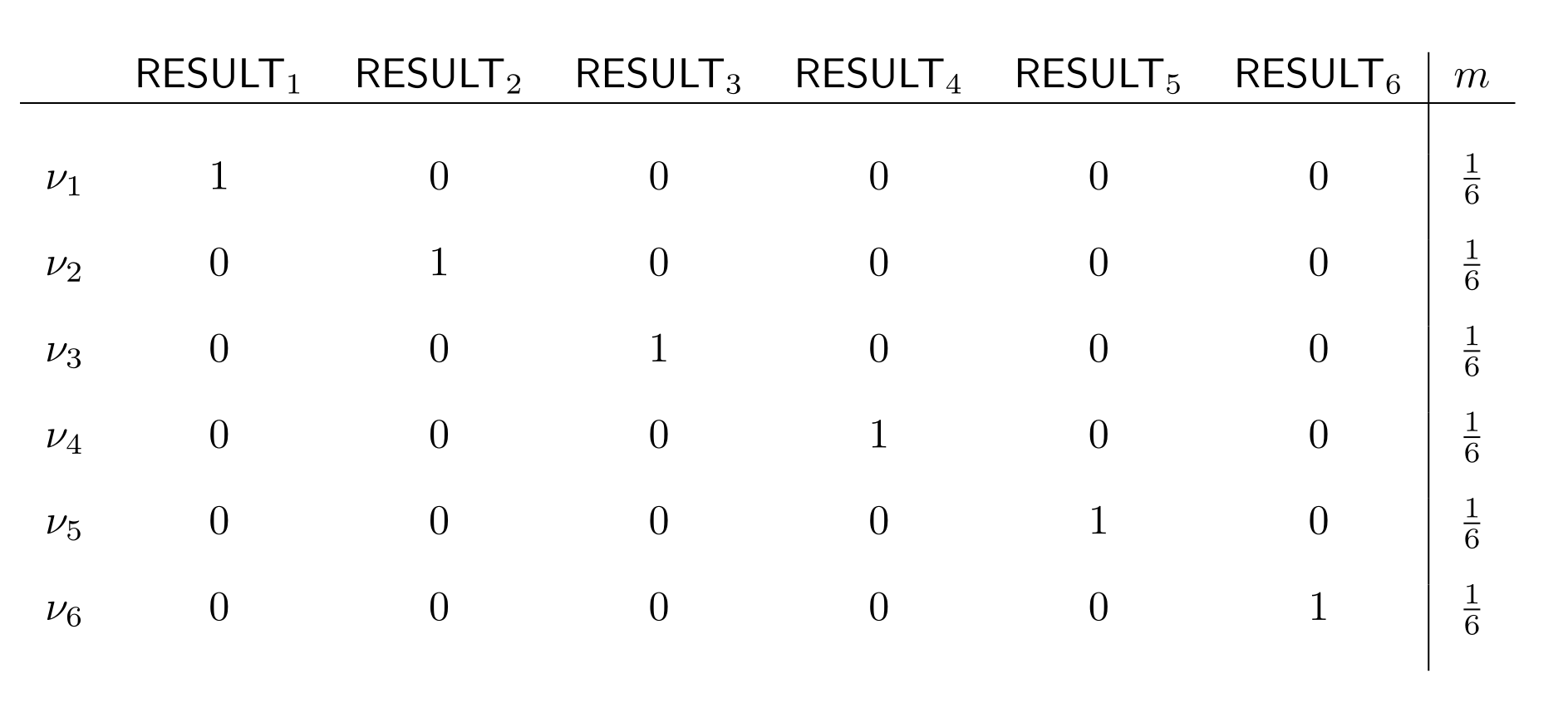
Let’s look at a simple, concrete example to see how this works. Remember our fair die from the last chapter?

In this setting, how would a Bayesian respond to getting the partial information that the die-roll was even, formalized as
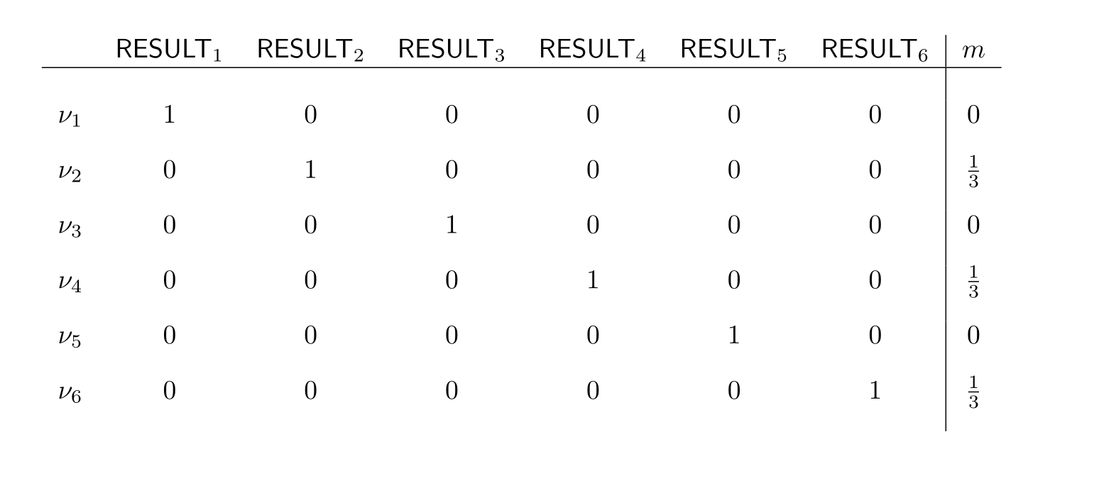
The answer is to conditionalize on this proposition. Let’s go through the outcomes of this. We’ve already calculated result for \mathsf{RESULT}_2 (abbreviated as \mathsf{R}_2) last chapter . The calculation, for \mathsf{R}_4 and \mathsf{R}_6 is exactly analogous, giving us:
In the case of \mathsf{R}_1,\mathsf{R}_3 and \mathsf{R}_5—the odd results—the calculation is also analogous in all three cases. We do the one for \mathsf{R}_1:
This holds because the only valuations where this formula is true are ones where both \mathsf{R}_1 and one of either \mathsf{R}_2,\mathsf{R}_4, or \mathsf{R}_6 is true. But all of these valuations have weight 0, meaning that the whole formula has value 0.
From this it immediately follows that:
Analogously, we get:
We can present the result in the following table:

This is as we should expect: when we learn that the die-roll is even, all the odd results become impossible.
Bayesian updating is an impressively effective method for changing believes in the light of evidence. The method has a lot of applications in AI, ranging from text classification to email spam filters.
We conclude this chapter by discussing the most important method for calculating conditional probabilities in practical settings, from which Bayesian updating receives its name: Bayes rule.
Bayes rule is a simple probabilistic law, which can easily be derived from the axioms of probability and states that:
There are alternative but equivalent formulations, such as:
The reason why Bayes rule is so important is because in practical applications the values on the right hand are often known or easier to figure out than the conditional probability on the left of the equation.
For example, if we’re wondering what should
Bayes formula tells us that this is the same as:
Our starting point was to say that
Now the point is that it’s easier to figure out what Pr(\mathsf{RAIN}\mid \mathsf{HIGH\_PRESSURE}) is easier to assess than Pr(\mathsf{HIGH\_PRESSURE}\mid\mathsf{RAIN}): high pressure makes rain unlikely, since low pressure is one of the main factors in rain. Let’s suppose we have:
Now all we need is to figure out what the unconditional probability of high pressure is. Assuming that it’s winter, when the air pressure is usually high, we could set:
The outcome would be
In this setting, we usually give the terms Pr(A\mid B), Pr(B\mid A), Pr(A), and Pr(B) special names:
-
Pr(A\mid B) is the posterior probability, since it’s the outcome of our learning process
-
Pr(A) is called the prior probability, since it’s what we know about the probability of A before learning that B
-
Pr(B) is called the marginal probability
-
Pr(B\mid A) is called the likelihood, since it’s a measure of how likely the thing we learned is. This concept connects Bayes formula to Bayesian statistics, but unfortunately, we don’t have the time to explore this connection here.
Logic-based learning in AI
This chapter was a brief overview of how learning in logic-based AI can work. But, as your doubtlessly aware, logic-based learning is not the standard paradigm for machine learning: statistical methods reign supreme.
The main reason for this is the computational complexity of logic-based learning procedures. This point is easy to see with the methods we’ve discussed in this chapter: AGM belief revision requires a defining a selection function that generally performs the contractions (removing the \neg A) and therefore needs to go through all the subsets of our knowledge base.
Bayesian updating, instead, requires updating the probabilities of every proposition, even if they’re not relevant to the learning situation.
Statistical machine learning are way more efficient in the model parameters they update.
But that doesn’t mean that logic-based learning methods have no place in AI: while they are not efficient as a general learning algorithm, they are useful methods when precision counts or the scenario allows for simple retraction functions or modeling with few propositions.
Last edited: 23/10/2024