Many-valued logics

In classical logic, we assume that every formula is either true or false. This is known as the principle of bivalence. While the assumption is valid in many contexts, it is clearly an idealization in others. Think of statements about the future, like “it will rain tomorrow”. Unless you’re a die-hard fatalist, you probably don’t think that statement is true or false now—its truth or falsity will be decided tomorrow. Or think about vague concepts, like warmth. Is 25°C warm? What about 21, 20, 19°C? Is there a clear cut-off point? If so, where? Is it at 20°C, maybe? Does that then mean that 19.999°C is no longer warm?—It seems that warmth is something that comes in degrees: 25°C is warmer than 22°C is warmer than 19°C. Examples like these motivate the study of many-valued logics, which abandon bivalence.

It turns out that non-bivalent reasoning is relevant in many different AI contexts. Just think of reasoning with incomplete information or robotic sensing. In this chapter, we’ll explore two non-bivalent reasoning systems, which are particularly important in AI-research:

• the 3-valued logic of Kleene, and

• the infinitely many valued fuzzy logic of Łukasiewicz.

As you will see, these systems figure in AI-technologies in different ways. We’ll see how Kleene’s logic, for example, is the basis for how SQL handles incomplete information, while fuzzy logic is used in industry products such as Automatic Train Control-systems for subway trains. Of course, we’ll only be able to scratch the surface of the field of many-valued logics, but you’ll add some very useful techniques and insights to your logical toolbox.

At the end of the chapter, you will be able to:

• explain the 3-valued Kleene truth-tables for negation, conjunction, and disjunction and their relevance to DBs

• test inferences for validity in Kleene’s 3-valued logic using a truth-table method

• explain the infinitely-valued Zadeh-operators for interpreting the negations, conjunctions, and disjunctions of fuzzy propositional variables

• formulate fuzzy rules to describe the interaction of fuzzy propositional variables, and explain their relevance to AI-systems.

Kleene Algebra

Recall our simply country DB from when we explored the relation between open FOL formulas and SQL queries. The content of the DB was given by the following tables:

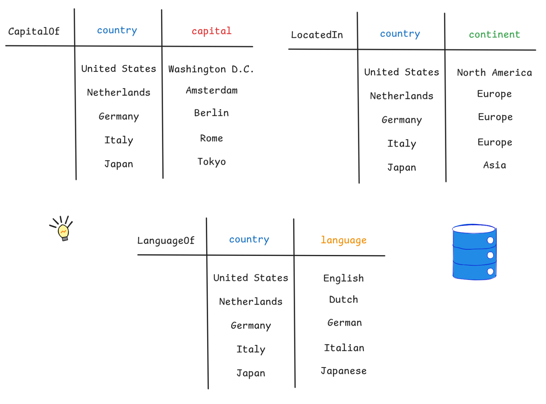
Now suppose that we learn of a new country. Let’s take Zimbabwe, for example, which is located in Africa and whose capital is Harare. But let’s suppose we don’t know which language(s) are spoken in Zimbabwe. In SQL, we can INSERT this information into our DB using the special marker NULL represent the “missing” information like so:

1
2
3
4
5
6
7
8

INSERT INTO CapitalOf VALUES
  ('Zimbabwe', 'Harare');

INSERT INTO LocatedIn VALUES
  ('Zimbabwe', 'Africa');

INSERT INTO LanguageOf VALUES
  ('Zimbabwe', NULL),

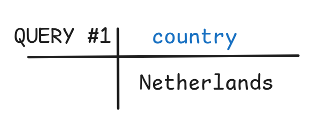
Now, let’s query the database and to ask for the countries which speak Dutch. Following the ideas we’ve discussed before, we can do this with the following query:

1
2
3

SELECT country
FROM LanguageOf
WHERE language = 'Dutch';

The return value is, as expected, the table with the single row Netherlands:

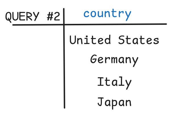
But now, let’s query our DB for the countries that dont speak Dutch:

1
2
3

SELECT country
FROM LanguageOf
WHERE NOT language = 'Dutch';

The return values are all the countries of which we know that they speak a language other than Dutch:

You can check this out yourself in our updated db-fiddle.

But what happened to Zimbabwe? It returns in none of the two queries and, in a sense, that’s to be expected: our DB doesn’t know whether they speak Dutch in Zimbabwe, so it neither returns the country as one where they do or where they don’t. But if we look at this from a logical perspective, things get a bit less clear.

Remember that SQL queries correspond to open FOL formulas and the return value for a query is the extensions of the extension of the corresponding formula in the model expressed by the DB. Now, in our toy example, QUERY #1 corresponds to the following formula:

In fact, the table above gives the extension of this predicate in our DB model.

A natural thought would be that the formula that corresponds to QUERY #2 is:

But something’s off here! Assuming classical logic, the fact that Zimbabwe wasn’t returned for Query #1 means that the truth-value of LanguageOf zimbabwe dutch is 0. In fact, our table doesn’t say that Dutch is the language of Zimbabwe. But since in classical logic, we interpret ¬ via the Boolean NOT, we have that:

That means that:

But QUERY #2 didn’t return Zimbabwe. So we seem to have that Zimbabwe is neither in the extension of LanguageOf x dutch nor in the extension of ¬ LanguageOf x dutch. Something went wrong.

What’s going on is that the NOT in our query is simply not the negation of classical logic. In fact, it is the negation of Kleene’s 3-valued logic, which is also known as K3.

By the way, note that there isn’t a contradiction here between the correspondence we established earlier between open formulas of classical FOL and SQL queries. In the construction we used in the exercises, we expressed negation using a WHERE NOT EXISTS construction. In our case, this would be:

1
2
3
4
5
6
7
8

SELECT country
FROM LanguageOf AS outer
WHERE NOT EXISTS (
  SELECT *
  FROM LanguageOf
  WHERE country = outer.country
    AND language = 'Dutch'
);

If you copy and paste this code into our db-fiddle, you’ll see that this query does return Zimbabwe as expected.

So, let’s explore the basic theory of K3 from a logical perspective and look at some other applications. For the purpose of this chapter, we’ll restrict ourselves to propositional K3. It’s rather straight-forward to extend the ideas to FOL formulas and you’ll explore some of these ideas in the exercises.

K3 allows for three possibilities: a formula can be true, false, or unknown, where the unknown truth-value corresponds to the SQL-marker NULL. The values true and false are represented as 1 and 0 as before. To represent the unknown value, we’ll use ω, which is how NULL is typically represented in database theory. So, the Kleene truth-values are:

Just like in Boolean algebra, there are different interpretations of these values. The interpretation we’ve been using so far is informational:

• the value 1 represents the information that something is true,
• the value 0 represents the information that something is false, and
• the value ω represents the lack of information.

But other interpretations are possible, such as decided for, decided against, undecided or high voltage, low voltage, intermediate voltage, etc. Even completely different interpretations, where ω means both true and false are possible. This leads to paraconsistent logic, which we won’t go into the details of here.

Also the notion of truth-function generalizes nicely from Boolean algebra to our Kleene algebra: Kleene truth-functions are functions that take our three values as inputs and outputs.

The standard Kleene truth-functions are given by the following tables:

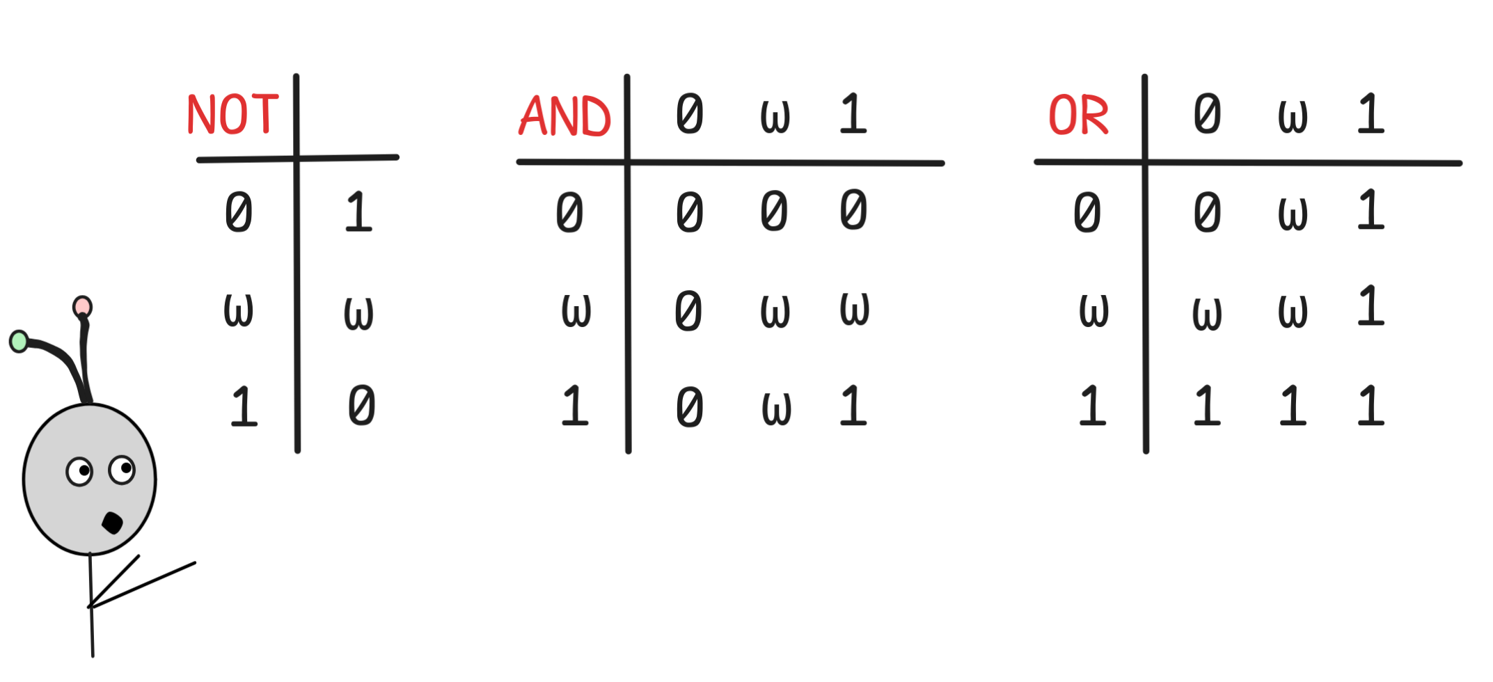
We denote these functions using NOT, AND, OR (in red) rather than NOT, AND, OR (in blue) to distinguish the Boolean from the Kleene truth-functions.

To understand the functions, our informational interpretation is helpful. For example, if we have the information that a sentence is false, i.e. has value 0, this is enough information to know that it’s negation is true, so we set NOT 0 = 1. But if we have no information about the sentence, i.e. value ω, then this is not enough information to determine what the negation of that sentence should be. In other words NOT ω = ω. This interpretation works for all the other connectives: if the information about the inputs is enough to determine the classical truth-value of the output, this is returned, otherwise ω. Note that, in particular, if the inputs are classical truth-values 0 or 1, the output of any Kleene truth-function is the same as the output of the corresponding Boolean function.

In contrast to Boolean algebra, in a Kleene setting, the functions NOT, AND, OR are not truth-functionally complete. To get a truth-functionally complete set, we need to add the following function, which is sometimes called the “definedness” function:

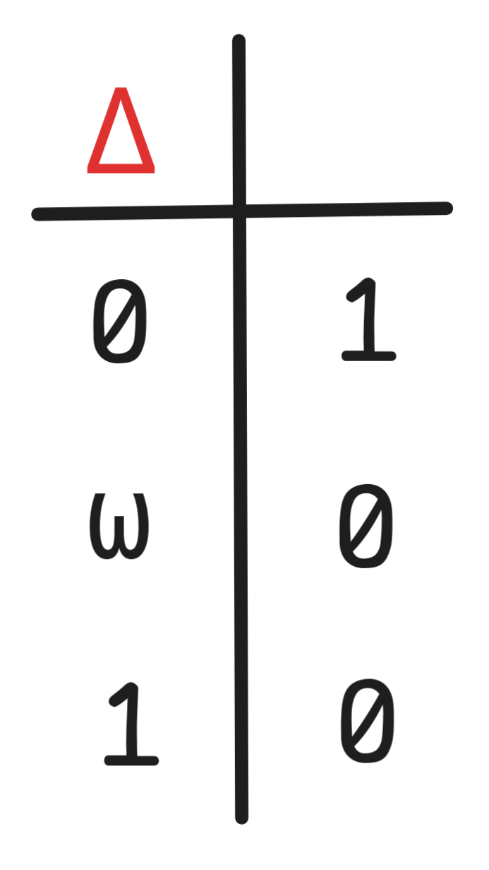
This function doesn’t play a huge practically role, but it cannot be expressed using NOT, AND, OR alone. But Δ together with NOT, AND, OR can express all possible Kleene truth-functions.

In Boolean algebra, we provided implementations of the Boolean truth-functions using relay circuits. In Kleene logic, an implementation are SQL queries using the SQL operations NOT, AND, OR. To show how this works, let’s create a simple SQL DB that contains two tables, one for all the Kleene values and one for all pairs of Kleene values:

 1
 2
 3
 4
 5
 6
 7
 8
 9
10
11

CREATE TABLE TruthValues (X BOOLEAN);
CREATE TABLE ValuePairs (X BOOLEAN, Y BOOLEAN);

INSERT INTO TruthValues VALUES
    (1),
    (NULL),
    (0);

INSERT INTO ValuePairs VALUES
 (1,1), (1,0), (0,1), (0,0),
 (1,NULL), (NULL,1), (NULL,0), (0,NULL), (NULL,NULL);

In that DB, the following queries directly reproduce our Kleene truth-tables:

 1
 2
 3
 4
 5
 6
 7
 8
 9
10
11

SELECT X,
	(NOT X)
FROM TruthValues;

SELECT X, Y,
    (X AND Y)
FROM ValuePairs;

SELECT X, Y,
    (X OR Y)
FROM ValuePairs;

You can convince yourself by running the code in db-fiddle.

A cool little side-effect of this is that you can use SQL as a K3 SAT-solver, which is an idea you’ll explore in the exercises.

Just like in Boolean algebra, there are laws of Kleene algebra. Here’s a straight-forward

This set of laws is a sound and complete axiomatization of Kleene algebras, that is we can derive all (and only) the laws of Kleene algebra from them.

Kleene Logic — K3

So far, we’ve been thinking about a low-level implementation of Kleene reasoning, viz. information retrieval from DB with incomplete information. But we can also use K3 for high-level deductive inference in situations with partial information or events with unknown outcomes, such as tomorrow’s weather.

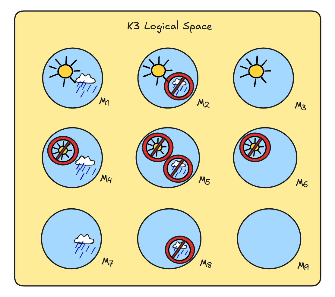
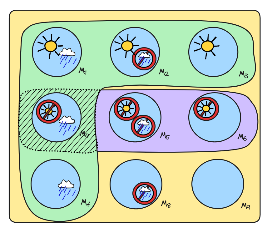
In order to do so, we need to define the notion of a model in K3. Remember that a model is just a possible reasoning scenario. Following along with the information idea, we can think of the different reasoning scenarios as information states. So, if we have, for example, two propositional variables RAIN to say that it rains tomorrow and SUN to say that tomorrow the sun will shine, there are now 9 scenarios:

1. We have the information that the sun will shine and that it will rain
2. We have the information that the sun will shine and it won’t rain
3. We have the information that the sun will shine but no information about rain
4. We have the information that the sun won’t shine and that it will rain
5. We have the information that the sun won’t shine and it won’t rain
6. We have the information that the sun won’t shine but no information about rain
7. We have no information about the sun but that it will rain
8. We have no information about the sun but that it won’t rain
9. We have no information about either the sun or the rain

That is, logical space looks something like this:

Following essentially the same idea as in Boolean algebra, we can think of each of these scenarios as a function from the propositional variables into the Kleene truth-values. The information state 1., for example, corresponds to the function that assigns both SUN and RAIN the value 1, while state 3. assings SUN the value 1 and RAIN the value ω. So, we can write v(A) just like before, just that v(A) { 0, 1, ω } rather than just {0, 1}.

The truth-values for complex formulas, then are calculated using the K3 truth-functions in the obvious way:

v( A) = NOT v(A)

v(A B) = v(A) AND v(A)

v(A B) = v(A) OR v(A)

Correspondingly, we also get the notion of a proposition expressed by a formula. In fact, the following definition works just like before:

A = { M : A is true in M }

These propositions are a bit “bigger” than the classical propositions, since there are now more models, but otherwise things work like in classical logic. Here are, for example, the propositions SUN and SUN RAIN :

In fact, we can also apply our general blueprint for the definition of logical consequence in K3:

P₁, P₂, … C   if and only if   P₁ P₂ … C

We can use this definition, for example, to see that our disjunctive syllogism from before is K3-valid:

(SUN RAIN), SUN RAIN

We can check this by inspecting the following diagram:

The shaded area is the intersection of SUN SUN RAIN of SUN and SUN RAIN . And the only model in that intersection is the one where we have the information that there’s no sun but it will rains, which is a member of RAIN . So, the inference is valid: from the information that it will be rainy or sunny and that it will not be sunny, we can infer the information that it will be rainy.

The fact that we get Disjunctive Syllogism in K3 also means that if we interpret the conditional

A B

v(A B) = (NOT v(A)) OR v(B),

we get a material conditional that satisfies MP. That means, in turn, that we can use forward chaining and backward chaining with Horn-clauses also in K3. That is, we can use K3 to reason with KBs in the context of potentially incomplete information. Great!

So, you might be wondering what’s the difference to classical logic, then? It turns out that there are inferences that are classically valid but invalid in K3, but it’s more instructive to think about tautologies first, which are the logical truths of propositional logic—formulas which have the value 1 in every model. In classical logic, there are plenty of tautologies, such as any formula of the form A A. But, as it turns out, there are no tautologies in K3. We won’t prove this general fact, but we can check a simple counter-example of a formula, which is a classical tautology, but not true in some K3 model.

Take the following formula, for example:

RAIN RAIN

v(RAIN RAIN) = ω OR (NOT ω) = ω OR ω = ω

But ω ≠ 1, which means that in any such model, where v(RAIN) = ω, is a model where RAIN RAIN doesn’t have value 1. Under the information interpretation, this makes quite some sense: it’s not the case that regardless of which information we have, we either have the information that it rains or the information that it doesn’t. There are no things that we know independent of any information.

There are classically valid inferences, which rely on the fact that statements like RAIN RAIN are tautologies, and which fail in K3. For example, the somewhat random inference:

SUN RAIN RAIN

If we take a model, where v(SUN) = 1 and v(RAIN) = ω, we’ve got a countermodel.

Unfortunately, though, the connection between SAT and logical consequence that we’ve used in Boolean logic and classical FOL doesn’t hold in K3:

P₁, P₂, … C   if and only if   not-SAT { P₁, P₂, …, C }

The reason for this is that there in K3, there can be countermodels that don’t satisfy { P₁, P₂, …, C }. A K3 countermodel is a model where all the premises are true, but the conclusion isn’t. But that doesn’t mean that the conclusion is false—it could also be a model where the conclusion is undetermined.

The model which shows that RAIN RAIN doesn’t follow from SUN in K3, is a case in point: it’s a model where RAIN, and thus RAIN RAIN is ω. But crucially, the negation of RAIN RAIN, that is (RAIN RAIN), is unsatisfiable—and so is every set that contains it, like

{ SUN, (RAIN RAIN) }

(RAIN RAIN)

RAIN RAIN

RAIN

{ SUN, (RAIN RAIN) }

But that doesn’t mean that we can’t use a SAT-solving style approach. For example, it’s straight-forward to develop a brute-force truth-table method, where we generate all the relevant models and check if in the models where the premises are true, the conclusion is as well. In fact, we can easily illustrate the idea in SQL.

Take our truth-value DB and consider the following query:

1
2
3
4

SELECT *
FROM TruthValues
WHERE ((X OR (NOT X)) = 0 )
	  OR ((X OR (NOT X)) IS NULL ) ;

This query returns all the rows of the table where the Kleene expression

either returns the value 0 or ω. But that’s just the truth-condition for the formula RAIN RAIN where we let v(A) = X. In other words, the query searches for a countermodel to the formula RAIN RAIN. It does find one, and so we can conclude that the formula is not a K3 tautology.

In a similar way, we can test the inference

SUN RAIN RAIN

using the SQL code:

1
2
3
4
5

SELECT *
FROM ValuePairs
WHERE ( Y = 1 )
	  AND (((X OR (NOT X)) = 0 )
	  OR ((X OR (NOT X)) IS NULL )) ;

You can see for yourself in our db-fiddle.

To conclude our discussion of K3, let’s talk about why K3 is a useful logic in AI-reasoning contexts. We’ve seen that it is intimately connected to low-level information retrieval—queries—with incomplete DBs. But there’s also a high-level connection to popular AI-reasoning methods we’ve discussed before.

Think about forward chaining and backward chaining with KBs containing Horn-clauses, for a moment. Remember our example of a KB for rainbow sightings:

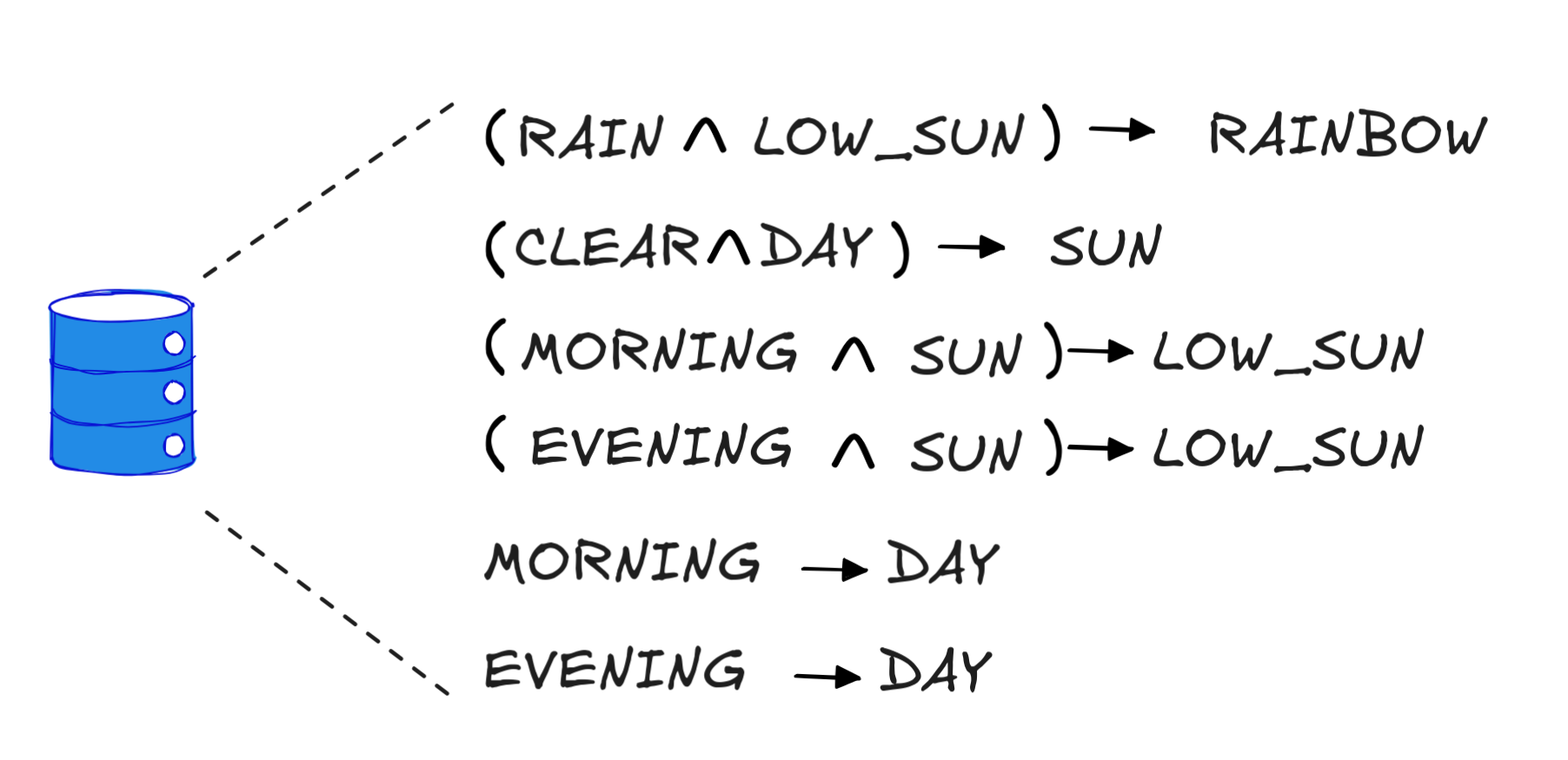
We managed to derive RAINBOW from this using the facts RAIN, MORNING, and CLEAR. In that situation, we concluded that RAINBOW is true—IA   will see a rainbow. But we also wondered what we should say if we couldn’t derive RAINBOW—for example, because our facts only contain RAIN, MORNING. Does that mean that we won’t see a rainbow or that we don’t know whether we will?

That depends on the way we interpret our KB: Is it a omniscient collection of all the laws and rules concerning the subject matter—say, all the ways a rainbow can occur? Then, we might be tempted to think that the fact that we can’t derive RAINBOW means that RAINBOW is false. In AI, this is known as the closed-world assumption.

But if our KB is more of a collection of our best understanding of the subject matter—which may be “gappy” and fail to contain all the true rules, then the story is different. We’d be doing logical predication under partial uncertainty, and the fact that we can’t derive RAINBOW would simply mean that we don’t have enough information to affirm that RAINBOW. If we also can’t derive RAINBOW, this would be a very good reason to assign RAINBOW the value ω—we don’t know! This is closely related to the so-called open-world assumption in AI. And for reasoning with KBs—for example as in expert systems like ours—the logic K3 is ideally suited.

Fuzzy Predicates

Vagueness is a very different motivation for dropping bivalence and is one of the main motivations for fuzzy logic. To illustrate the idea, think about which temperature means “warm” again. A standard and natural way of thinking about it is to say that warmth comes in degrees, which we can measure by a number between 0—meaning definitely not warm—and 1—meaning definitely warm. So, 0.75 warm means something like definitely more warm than cold, but not all the way there, while 0.1 warm means not freezing cold, but also barely warm.

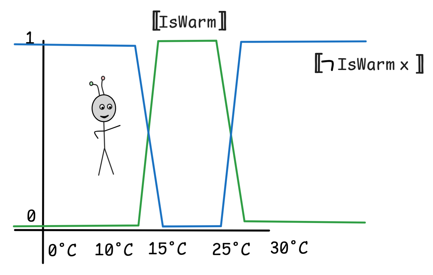
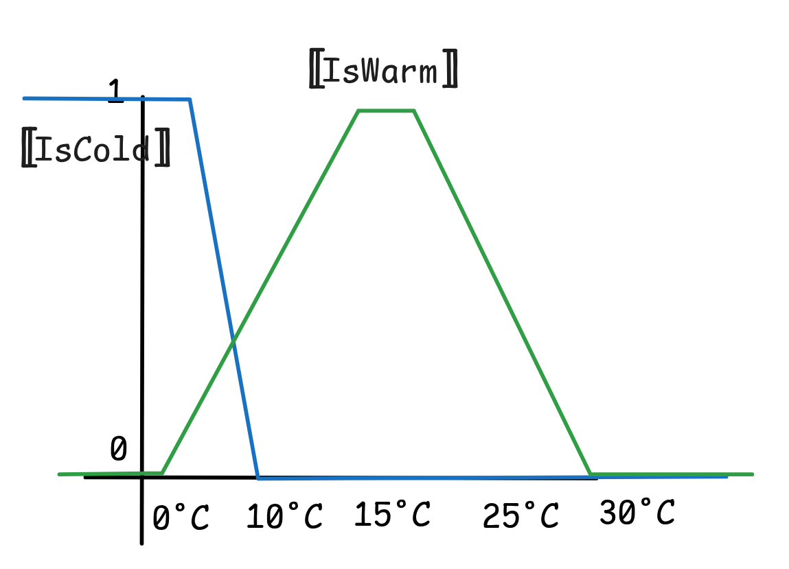
If we take this idea seriously and assume a language with three predicates IsCold, IsWarm, and IsHot, we can assign those predicates values between 0 and 1 when applied to a temperature in order to represent the extend to which this temperature is considered cold, warm, or hot. One way of assigning such values is represented in the following diagram:

This is the idea of fuzzy predicates: we’ve treated IsCold, IsWarm, and IsHot as fuzzy predicates of temperature. In contrast, the binary predicates of classical FOL are also called crisp predicates.

Fuzzy logic deals with inference involving fuzzy concepts. While it is central for many AI-technologies, especially so-called fuzzy control systems, which you find in automotive systems (trains, cars, plains, etc.) or self-regulating thermostats, it turns out to be rather difficult to formulate theory of high-level inference with fuzzy predicates—difficult, though not impossible. Accordingly, we’ll only scratch the surface of fuzzy logic in this chapter, but we’ll illustrate some basic ideas of working with fuzzy predicates, which will come in handy if you ever get your hands dirty with fuzzy AI systems.

For this purpose, we’ll work with the language of FOL but without the quantifiers. For simplicity, we’ll also ban function symbols. That is, for us, the expression

is a well-formed formula, but

x(x ≥ 10°C IsWarm x)

is not.

A fuzzy valuation for such a language is defined very similarly to an FOL model: we have a (non-empty) domain, D, and denotations a D for all the constants. The main difference to an FOL model is that for the predicates, we don’t assign extensions in the usual sense—that is sets of objects having the described property—but we associate with each predicate Pⁿ a function Pⁿ , which assigns to all n inputs from the domain a real number between 0 and 1 (inclusive). This number measures the extend to which the predicate applies to these objects.

That is, if our domain contains all the temperatures, then

IsWarm 10°C = 0.01

means that in our model 10°C is barely warm. In fact, we’ll continue working with temperature examples, so we’ll just assume that our domain D contains all the temperatures and our language has a name for each such temperature: 10°C for 10°C, 12.75°C for 12.75°C, and so on. That is, our models look like the diagram above. The extension of the predicates IsCold, IsWarm, and IsHot in such a model, then, is given by curves like the colored ones depicted.

The value of an atomic ground formula in such a model is easily defined. We say, for example, that:

IsHot t = IsHot t

t

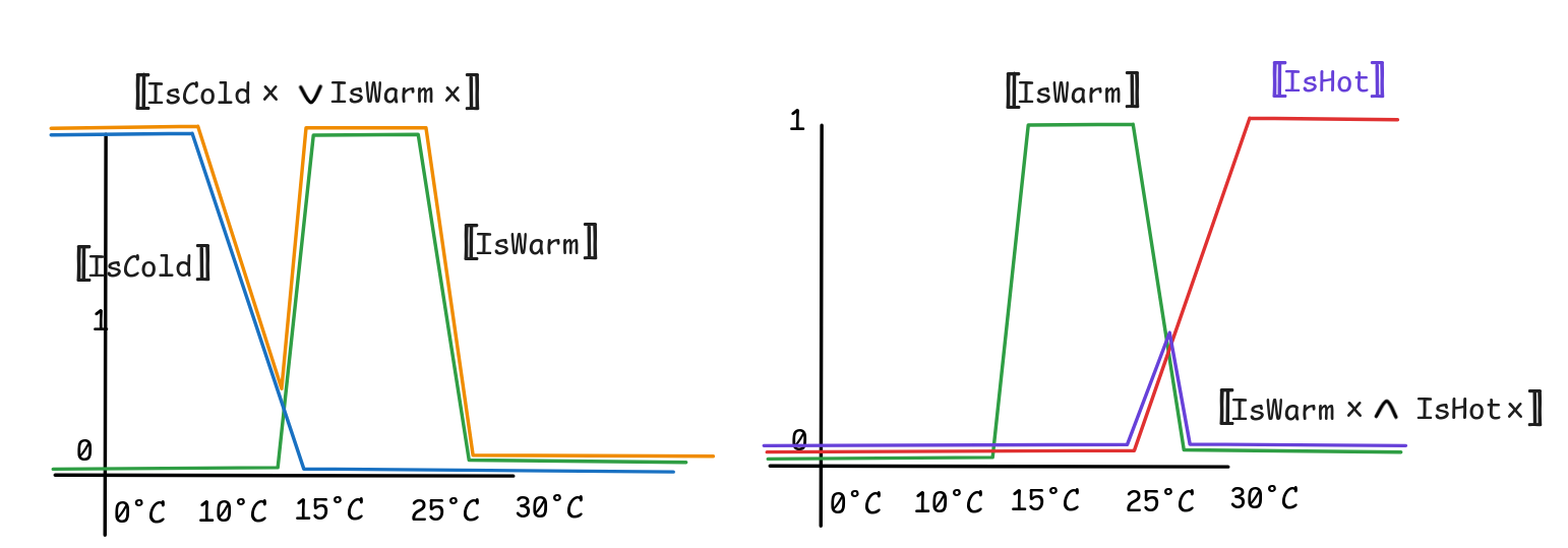
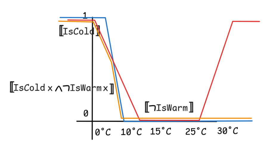
The main question we’ll be looking into now is how we can interpret complex fuzzy expresions in such models. What, for example, is the value of the following complex open formula:

IsWarm x IsCold x

We want it to be a fuzzy function over the domain, but which one?

The standard way of interpreting such expressions is using the so-called Zadeh-operators, which are named after Lotfi Zadeh, who introduced fuzzy logic to AI-research—even though their logic has already been studied by Łukasiewicz.

The idea is that we can say:

A = 1 - A

A B = min A B

A B = max A B

Here, min and max are the minimum and maximum function respectively, which return the biggest value among their inputs in the case of max and the smallest input in the case of min.

To see how these work, it might help to look at the outcomes of these operations in the fuzzy model we’ve described above:

In these models, there is also a natural notion of deductive consequence, which has already been explored by Łukasiewicz in the 1920s. The idea is that, for example, IsCold 10°C entails, in a sense, IsCold 10°C IsWarm 10°C since the value of the latter is always at least as high as the value of the former.

More generally, we say that a premise set P₁, P₂, … fuzzy entails a conclusion C just in case for every model, the minimum of the values P₁ , P₂ , … is smaller than or equal to the value C , that is:

P₁, P₂, … C   if and only if, in all models, min { P₁ , P₂ , …} ≤ C

At face value, this definition doesn’t satisfy our blueprint for deductive validity, but using the concept of a T-norm it can be brought much closer to that pattern. But for now, we focus on the above formulation since it gets us much closer to so-called fuzzy rules, which are the basic building block of fuzzy control systems.

Fuzzy Rules

A fuzzy rule is, in essence, a model constraint that enforces that some conditions—the antecedent of the rule—fuzzy imply (in the above sense) a conclusion. Typically, we formulate these fuzzy rules using open formulas of with appropriate free variables. For example, we write the fuzzy rule that IsHot fuzzy entails AcOn—where AcOn is a fuzzy propositional variable which just gets a fuzzy value assigned—either as

or using arrow notation as

IsHot x AcOn

We postulate that fuzzy rules have a kind of MP property where a model that satisfies a rule just in case for every object in the model, the value of the consequent of the rule applied to the object is at least as big as the value of the premise of the rule applied to it.

Some rules, like

IsHot x IsHot x IsWarm x

hold with mathematical necessity—simply because of how the operators are interpreted.

But other rules, we need to enforce. And that’s the idea of fuzzy control systems. Think, for example, of a self-regulating heating system, which aims to keep the warm always warm and cozy, never too hot and never too cold. One way of implementing such a system is by means of a fuzzy rule.

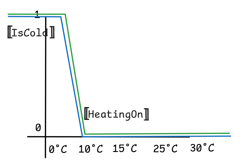
Suppose for the setup that we define our fuzzy predicate IsCold is given by the above diagram. Then we can implement our fuzzy heater by means of the following rule:

IsCold x HeatingOn

Here HeatingOn is again a fuzzy propositional variable, which simply gets a value between 0 and 1 in every model and which represents the extend to which the heating is engaged.

The idea is to enforce through some mechanism that this rule is satisfied by the temperature at any given point in time. That is, the system ensures that the extend to which HeatingOn is true at any time coasts the line IsCold:

These kinds of fuzzy control systems are industry standard in aviation, space-travel, train regulations, self-driving cars, heating systems, and many more places. One important advantage of such systems as compared to “crisp” systems is that they behave “smoothly”. A crisp thermostat just turns the heating on or off if the temperature falls below a certain threshold. This can be very uncomfortable if the temperature is set to 20°C, it falls to 19.9°C and all of a sudden the heating blasts on full power. A fuzzy control system will only turn the heating on a little bit at 19.9°C and then quickly off again. In this way, fuzzy systems can also be much more efficient than crisp control systems.

This efficiency can be even more noticeable, if we can adjust what IsWarm means for us. Suppose, for example, that we can set the curve for IsWarm as follows, while leaving IsCold unchanged:

Now, the fuzzy following fuzzy rule

IsCold x IsWarm x HeatingOn

will be more energy efficient than just:

IsCold x HeatingOn

since the former rule will stop heating quicker. Just inspect the following diagram:

This is just a small teaser of the huger world of fuzzy logic, but I hope it became clear that there are excellent low-level applications of these core logical methods.