Logical proofs

A logical proof is a chaining of inference rules applied to logical formulas, which models natural language step-by-step reasoning. We’ve already seen a simple example of a proof, when we discussed the chaining methods. The following structure, for example, is a logical proof that derives RAINBOW from the assumptions

MORNING, CLEAR, RAIN, MORNING DAY, (CLEAR DAY) SUN, …

… (MORNING SUN) LOW_SUN, (RAIN LOW_SUN) RAINBOW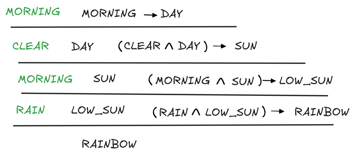

But the proofs we’ve seen so far are rather limited in scope: using genMP, we can only reason with conditionals where the antecedent is a conjunction of formulas. We can’t use it, for example, to infer WET from

(RAIN SWIM) WET

Systems for logical proofs, also called proof calculi, solve this issue by introducing principles and inference rules that can handle different kinds of inferences in one single system. The ultimate theoretical aim is to develop proof systems, which are complete in the sense that with their rules we can re-construct all valid inferences. Gödel’s completeness theorem—not to be confused with his incompleteness theorem—is one of the main achievements of 20th century logical theory.

Proof systems have their origin in mathematics: Euclid’s Elements is often credited with making rigorous proof the primary method of mathematical research. Especially since the 19th century, mathematicians have been paying special attention to proof systems in the context of the foundations of mathematics, where their study is aimed at solving issues concerning the very nature of mathematical thought. This is the birth of mathematical logic, which is the sub-discipline of logic that has gifted us results like Gödel’s incompleteness theorems and theories like set theory, which is ubiquitous in mathematics and the sciences.

But the use of proof systems has long transcended the realm of pure mathematics. Soon after they became the focus of logical attention, the relevance of proof systems to the theory of computation was discovered, leading to observations like the Curry-Howard correspondence, which establishes a direct relationship between logical proofs and computer programs. As such, the study of logical proofs is also part of the foundations of computer science. But also in AI-research specifically, applications abound.

There are, for example, applications that are perhaps best described as intelligence amplification (IA) rather than artificial intelligence (AI), even though the lines are a bit blurry here. The idea is that since logical proofs are rigorously defined mathematical models of natural language inference, we can use computational implementations of proof systems to check or verify our natural language inferences. This is the idea underlying proof assistants, which can guide and correct the process of developing logically valid proofs. In this chapter, you’ll learn about Lean, which is one powerful example of such a proof assistant.

Since proof assistants interface with their users in formal languages and genAI-systems, such as ChatGPT, Gemini, Claude, LLama, et al., are very good at learning formal languages, hybrid AI systems using an architecture involving LLM's together with proof assistants have yielded promising results in “artificial mathematics”—the project of developing human or super human-level AI-systems for logical and mathematical reasoning.

In fact, proof systems are the playground for a certain kind of automated theorem prover (ATP). State of the art ATP’s often use methods we’ve already discussed, such as resolution or SAT-solving. But there are also ATP’s which are expert systems for proof search, i.e. the activity of searching through logical proofs in well-designed proof systems, using knowledge bases that contain expert knowledge on logical proofs. An example of this approach is MUSCADET.

Today, these kind of expert system architectures are virtually extinct in ATP-contexts, but there’s an intriguing way of thinking about what’s going on in genAI-research on mathematical proofs in terms of proof search: effectively, LLM-based theorem provers are reasoning inductively about proofs, rather than deductively, like expert systems. But before we can go into more details, we need to better understand how logical proofs work in their standard applications.

At the end of this chapter, you will be able to:

• explain the concept of a formal proof in a calculus
• name important kinds of proof systems with their advantages and drawbacks
• construct logical proofs the natural deduction calculus for intuitionistic and classical propositional logic
• verify simple natural deduction arguments in the Lean proof assistant
• explain the core idea behind the Curry-Howard correspondence

Proof systems

Over the years, logical research generated many different kinds of proof systems. For the purposes of AI-research, you don’t need to know the ins and outs of all these different systems. But it is useful to have an overview of the most important kind of systems and their different use-cases. We’ll begin by reviewing the following important families of proof systems, highlighting their specific uses for AI purposes:

1. Axiomatic proof systems, such as Hilbert systems.
2. Structural proof systems, such as sequent calculi.
3. Algorithmic proof systems, such as tableaux-systems and resolution-style systems.

Then we’ll do a deep dive into a particularly import kind of proof system, which is both useful for practical reasoning with logical formulas and for AI applications, which are:

4. Natural deduction systems

As a running example for ours discussion, let’s consider the following inference in natural language, carried out by IA :

If it's windy or rainy, then I get cold, and if I get cold, I need my heating unit. I see that it's rainy. So, I need my heating unit.

The first step whenever we want to do anything using logical methods in natural language contexts is to represent the inference in a formal language using our by now familiar knowledge representation techniques. For the premises, we get:

((RAIN WIND) COLD)  (COLD HEATING)  RAIN

The conclusion is simply: HEATING.

So, the entire formal inference, therefore, becomes:

((RAIN WIND) COLD), (COLD HEATING), RAIN HEATING

Using our established methods, such as truth-tables or resolution, we can see that this inference is deductively valid:

((RAIN WIND) COLD), (COLD HEATING), RAIN HEATING

But in this chapter, we’re interested in a different perspective on the inference, namely how we can see its validity via step-by-step arguments. That’s what proof systems are for.

To say that there exists a formal, step-by-step argument from the premises to the conclusion, we use the symbol 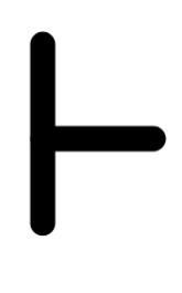, called the “turnstile”. So, in our example, we would write

((RAIN WIND) COLD), (COLD HEATING), RAIN HEATING

to say that there exists a step-by-step argument—a logical proof—from the premises to the conclusion.

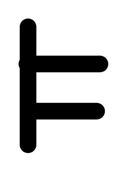
It’s important to realize that the symbols and say different things: the former, , says that an inference is valid; the latter, says that there exists a logical proof from the premises to the conclusion. We want the two to coincide, and in most systems they do. This is the content of the soundness and completeness theorems for a logic, which state that for all inferences:

P₁, P₂, … C   if and only if P₁, P₂, … C

Most logical systems you’ll come across in AI-application have this property, especially when we’re dealing with basic systems for classical propositional logic, like below. But it’s also important to know that there are logical systems where no complete proof system exists—where not for every valid inference there exists a step-by-step proof. An example is second-order logic.

Returning to our main topic, different proof systems have different ways of showing that:

((RAIN WIND) COLD), (COLD HEATING), RAIN HEATING.

Let’s check out how.

Axiomatic systems

Axiomatic systems are modelled after the approach of Euclid’s elements, which starts from basic laws or axioms and constructs logical proofs by deriving consequences using simple inference rules. In logical theory, axiomatic systems are typically called Hilbert system.

Here’s how a logical proof for our inference would like in a Hilbert system for propositional logic:

1. RAIN (Premise)
2. (RAIN (RAIN WIND)) (Axiom)
3. (RAIN WIND) (1., 2., MP)
4. ((RAIN WIND) COLD) (Premise)
5. COLD (3., 4., MP)
6. (COLD HEATING) (Premise)
7. HEATING (5., 6., MP)

Only one rule of inference is used in this derivation, namely MP, which is characteristic of Hilbert calculi. Typically Hilbert calculi have only one or two rules of inference and rely on the axioms to do the “heavy lifting”.

The only axiom in this derivation is 2. (RAIN (RAIN WIND)), which expresses the thought that if one disjunct is true the disjunction is true as well. The axioms of a Hilbert calculus for propositional logic are logical truths, that is formulas which are true in every model. The challenge when formulating a Hilbert calculus is to find a collection of logical truths of the logic, which allow for the derivation of all valid consequences. We’ve already encountered this idea Boolean algebra, where we looked at how to derive Boolean laws from others.

Here’s a list of axioms, which together with the rule of MP form a sound and complete Hilbert calculus for classical Boolean logic, where A,B,C can be any formula:

• (A (B A))
• ((A (B C)) ((A B) (A C)))
• (( B A) (A B))
• ((A B) A) and ((A B) B)
• (A (B (A B))
• (A (A B)) and (B (A B))
• ((A C) ((B C) ((A B) C)))

That is for all and only the valid inferences, we can derive the conclusion from the premises in this calculus.

As you can see in this example, Hilbert calculi are typically quite “compact”. They manage to compress a lot of logical information into a few basic axioms and a couple of inference rules.

While this is certainly memory efficient, it is terrible for automated reasoning. Proofs in Hilbert calculi are typically quite hard to find and can get unreasonably long.

Here’s an example to illustrate both points, by showing that the condition

RAIN RAIN

1. ((RAIN ((RAIN RAIN) RAIN)) ((RAIN (RAIN RAIN)) (RAIN RAIN)))

     (Axiom 2. with A = RAIN, B = (RAIN RAIN), and C = RAIN)

2. (RAIN ((RAIN RAIN) RAIN))

     (Axiom 1. with A = RAIN and B = (RAIN RAIN))

3. ((RAIN (RAIN RAIN)) (RAIN RAIN))

     (1., 2., MP)

4. (RAIN (RAIN RAIN))

     (Axiom 1. with A = RAIN and B = RAIN.)

5. (RAIN RAIN)

     (3., 4., MP)

While providing Hilbert-style logical proofs is certainly a learnable skill, it is not an easy thing to do—not even for computers. To find the above proof in an algorithmic fashion, one has to systematically search through all possible values that A,B,C could take in the axioms. Not a good starting point.

Hilbert calculi are a common starting point for logical inquiry in AI. For example, proof systems for modal logics, which are very important in more complex hardware and software verification settings, are typically presented Hilbert-style. The computationally more tractable approaches to proof systems that we look at next don’t work for some logics. Instead, Hilbert systems are the “tried and true” go-to method, which often yields the desired results.

Sequent calculi

Sequent calculi take a fundamentally different approach to logical proofs. Rather than directly working with formulas, they work with so-called sequents. Sequents are “meta”-statements of sorts, which are formal claims of valid inference using the sequent arrow, . For our example, then, the aim is to derive the following sequent:

RAIN, ((RAIN WIND) COLD), (COLD HEATING) HEATING.

Such a derivation will then be the proof corresponding to the claim that:

((RAIN WIND) COLD), (COLD HEATING), RAIN HEATING

Here’s how this works in a standard sequent calculus for classical propositional logic would derive this sequent:

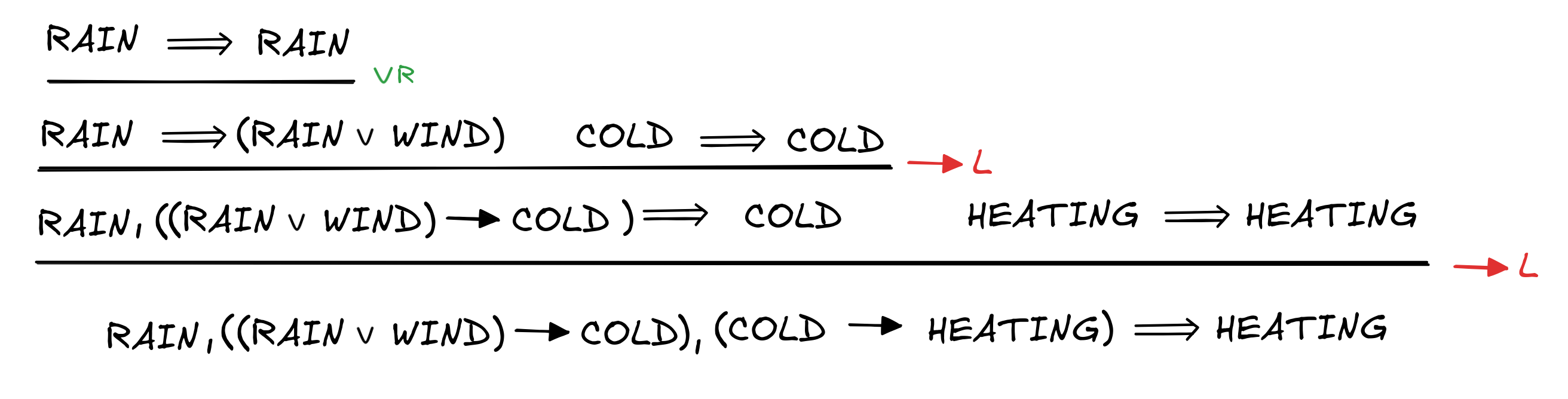
The derivation begins with RAIN RAIN, which is called an “initial sequent”—essentially an axiom of sequent calculus. These initial sequents express the basic logical fact that every statement logically entails itself: if it rains, then it rains. We could also think of this as a trivial inference.

From these kind of basic inferences, the sequent calculus proof constructs more complex sequents from the simple ones by applying sequent rules. For example, the inference from RAIN RAIN to RAIN (RAIN WIND) uses the rule R, which in general looks like this, where Γ is any collection of premises and A,B any formulas:

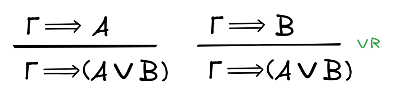
The idea of this rule is that if the Γ’s logically imply A, then they also logically imply (A B), since A implies (A B).

There are many different ways of constructing a sequent calculus for classical propositional logic, but one is this:

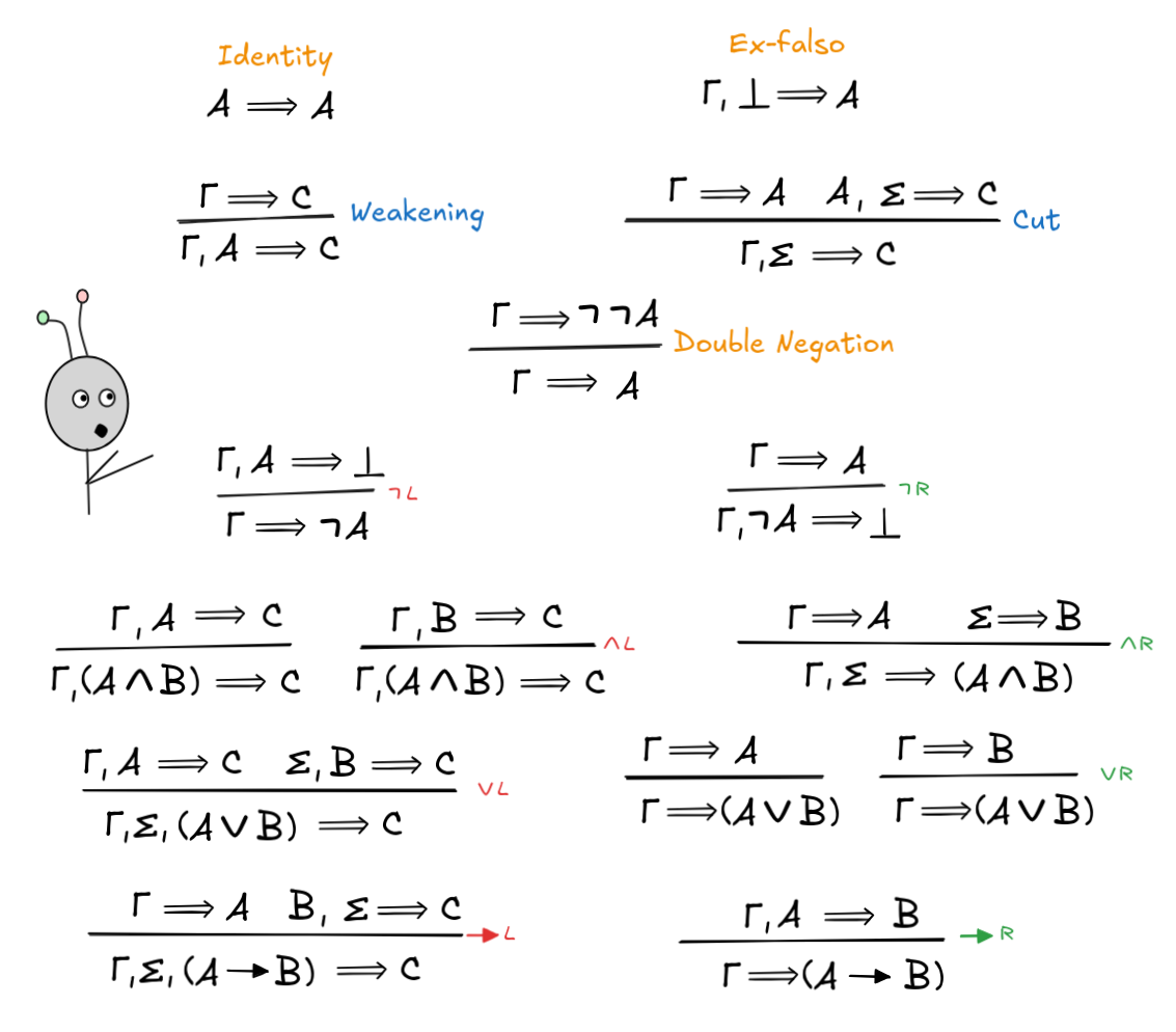
As you can see, there are a lot of rules here. For each logical connective there are rules that introduce the connective on the left side of (here in red) and rules that introduce the connective on the right side of (here in green). The so-called “left-rules” for a connective tell us what follows from a formula involving the connective based on the consequences of the formulas the connective is operating on. The “right-rules” for a connective, instead, tell us what a formula involving the connective follows from given what it’s parts follow from.

The symbol , which occurs in the rules for negation, for example, is a special “contradiction”-symbol, which is also called falsum. It is a special propositional variable which is false in every model. It is extremely useful in proof-theoretic contexts, where Γ, A says that we can derive a contradiction from A and Γ. From this we infer that the formulas in Γ must entail A.

Additionally, there are principles that express basic logical facts (here in orange), and so-called “structural” rules, which don’t involve any connectives at all (here in blue). So in contrast to Hilbert calculi, which have many axioms and few rules, in sequent calculi, we have few axioms and many rules. But these rules serve a specific purpose.

Together these rules allow us to recursively construct complex implications from simpler ones, as in the case of our example. In this way, sequent calculus proofs give us insights into how different valid inferences hang together or interact. This observation is the starting point for structural proof theory, which investigates how alternative formulations of the sequent calculus rules can help us better understand the nature of deductively valid inference.

From this perspective, the role of sequent calculi in logical research is primarily foundational. In fact, sequent calculi have been instrumental in the obtaining of fundamental results in mathematical logic, such as Gentzen’s consistency proof for the standard theory of natural numbers, which shows that you can’t prove in that theory mathematical falsehoods like 0 = 1.

In the context of AI-research, you will therefore mainly come across sequent calculi in foundational papers. But they are also useful for another reason: in contrast to Hilbert calculi, in sequent calculi, we can typically carry out efficient proof searches. The way this works is that from any sequent we’d like to prove, we can try to work backwards through the rules until we, hopefully, hit initial sequents. How well such proof searches work depends a lot on the concrete formulation of the calculus in question. But we shall not go into too much depth here, as the algorithmic systems we’ll move to next are more robust implementations of this idea.

Algorithmic systems

There are many different kinds of algorithmic systems, but many of them are SAT-based. That is, they are build on the idea we discussed before that we can reduce valid inference to the unsatisfiability of the premises with the negation of the conclusion:

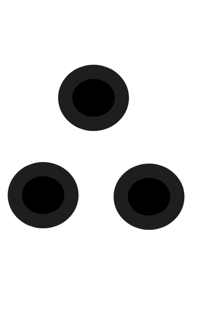
P₁, P₂, … C   if and only if not SAT { P₁, P₂, … , C}

The analytic tableau method works by recursively unfolding formulas according to their truth-conditions, producing a tree-representation of the possible ways those conditions might be satisfied. A tree in the mathematical sense is simply a structure of the following kind:

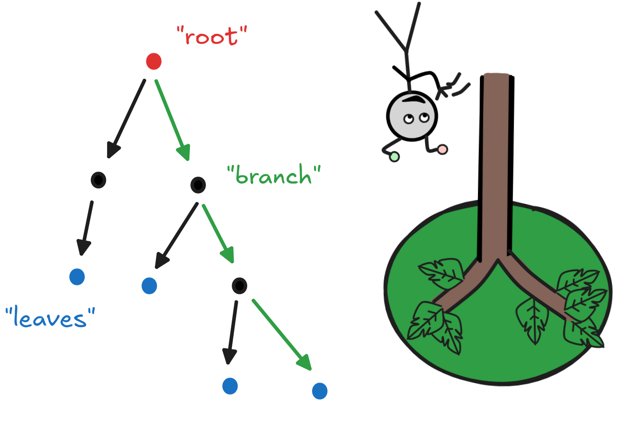
The circles are called nodes, the top-most node is the root (here in red), the outermost nodes are leaves (here in blue), and a way of getting from the root to a leave is called a path (like the green path from the root to the right-most leaf). It’s a defining characteristic of trees in the mathematical sense that there’s a unique path from the root to every leaf. By the way, our parsing trees from syntax-theory are also trees in this precise mathematical sense.

In a tableaux, the nodes are populated with formulas and each branch corresponds to a different way in which the formulas at the root could be true. Here’s how this looks like in our example inference:

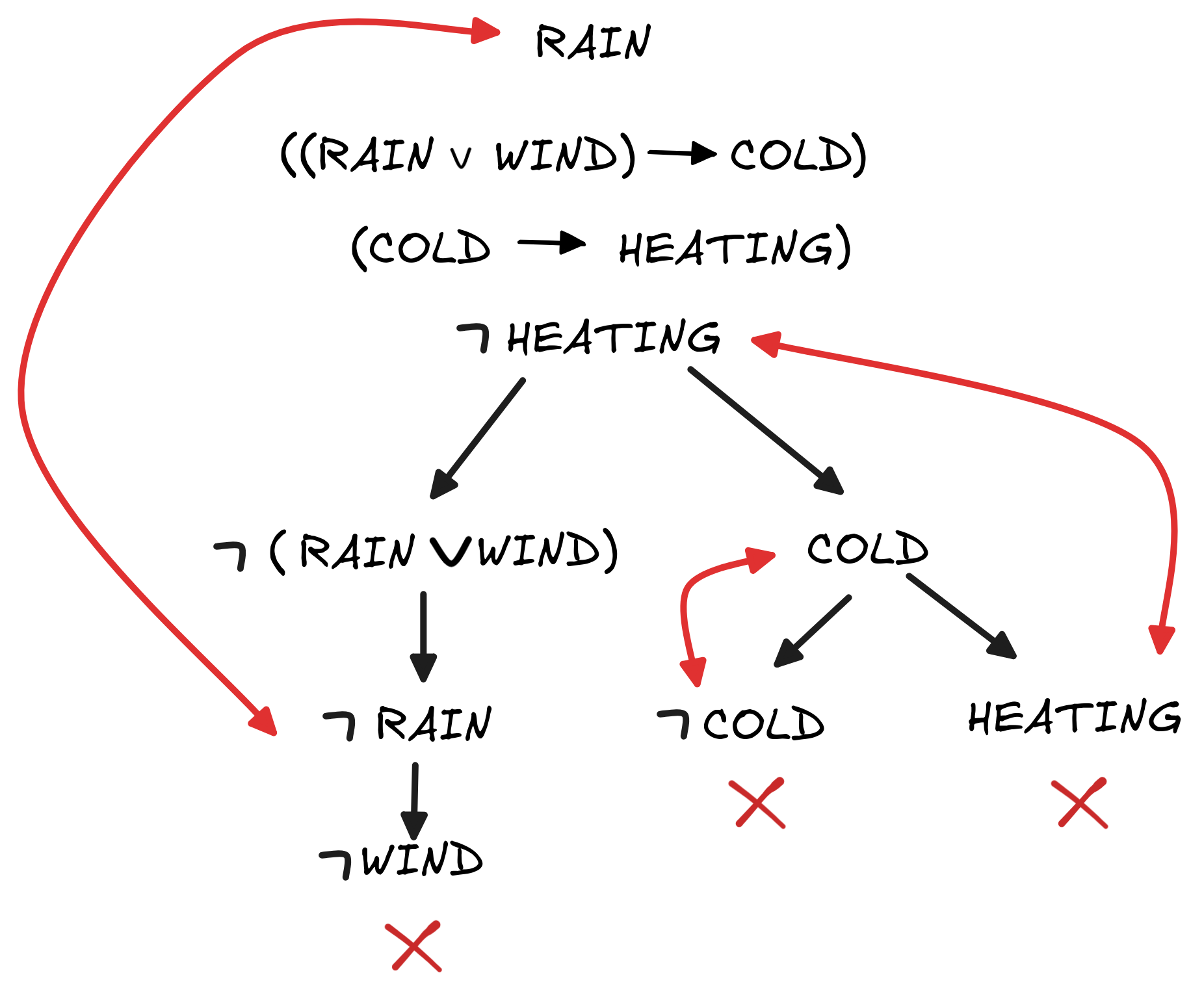
What’s going on here is that the we start with the premises and negation of the conclusion of our inference and then recursively unfold the truth-conditions for the formulas involved. For example, the first “branching” to the formulas (RAIN WIND) and COLD unfolds the two ways in which the conditional ((RAIN WIND) COLD) could be true. By our Boolean implementation of , we have:

v(((RAIN WIND) COLD)) = (NOT v(RAIN WIND)) OR v(COLD)

NOT v(RAIN WIND) = 1

NOT v(RAIN WIND) = 1

v( (RAIN WIND)) = 1

((RAIN WIND) COLD)

In a similar fashion, (WIND RAIN) gets unfolded to RAIN and WIND. If we assume that

v( (RAIN WIND)) = NOT(v(RAIN) OR v(WIND)) = 1,

RAIN

WIND

All the other tableau rules are motivated by completely analogous arguments. Here is a complete set for classical propositional logic:

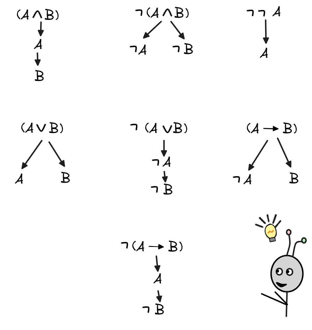
To generate a tableau, one simply recursively applies these rules by extending every branch that passes through the formula according to the rule.

If a branch contains a contradiction, it is eliminated—closed off as we say. If this happens to every branch in a complete tableau, like in our example, we consider this the proof that the formulas at the root aren’t jointly satisfiable—which means that the inference in question is valid. That is, the tableaux above is the logical proof that:

((RAIN WIND) COLD), (COLD HEATING), RAIN HEATING.

If there are branches that don’t close off, this shows that there exists a countermodel to the inference in question. Here’s a case where this happens, which shows that

((RAIN WIND) COLD), (COLD HEATING), SUN HEATING.

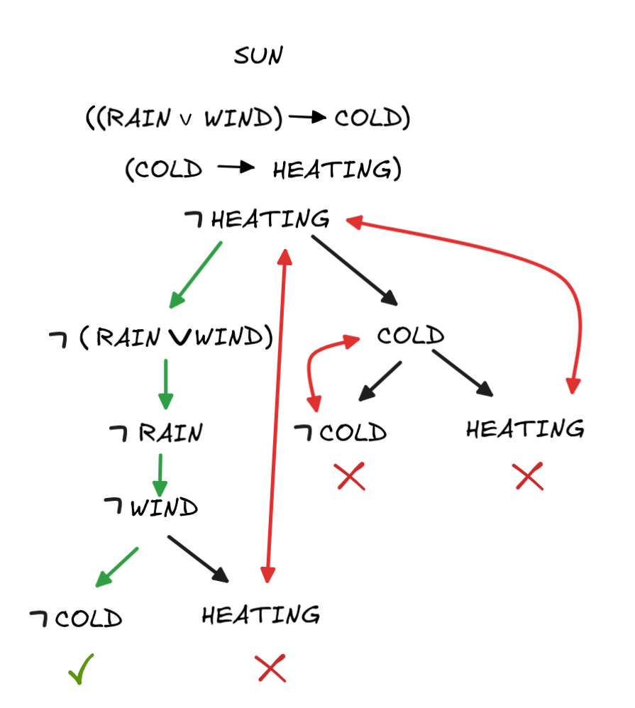
All rules have been applied and some branches close off. But the left-most one (here indicated in green) remains “open”. A great advantage of the tableau-method is that we can directly “read off” a countermodel from it. Here, the corresponding countermodel is given by

What makes tableau particularly fruitful for AI-research is their algorithmic nature: they are effectively an algorithm for countermodel search. Moreover, they can easily be made more efficient, for example, by checking for contradictions after each rule application, to eliminate branches early. Tableau systems that are optimized in this way are the basis for many ATP-applications.

The main drawback of tableau is that they are essentially SAT-solving algorithms in disguise. As a consequence, they are not very “natural” in the sense that it can sometimes be hard to see what’s going on in a given tableaux and it’s not straight-forward to go back and forth between natural language arguments and tableau proofs—they are simply not a great model of natural language step-by-step inference. This makes them less useful for use in proof assistants, for example, which are supposed to be formalized augmented intelligence systems that can help us verify our natural language inferences each step along the way.

Natural deduction

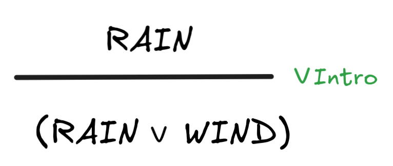
The system of natural deduction was specifically developed with rigorous natural language inference as a target in mind. The system has no axioms, only inference rules. The idea is that each inference rule corresponds to a basic natural language inference involving the connectives. Here’s how this plays out for our running example:

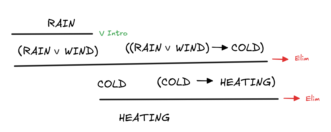
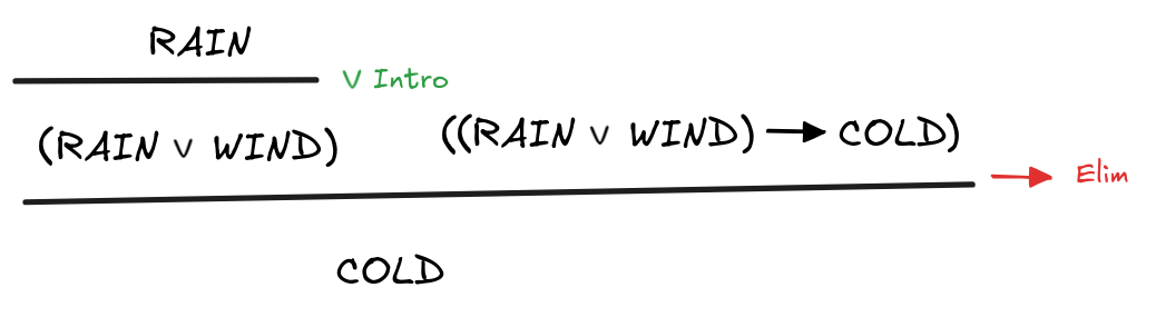
What’s going on here is that our premises are assumptions in a proof tree, where we apply inference rules to derive conclusions until we eventually bottom-out at our desired conclusion. There are rules that introduce connectives, like Intro, which we use to infer (RAIN WIND) from RAIN. Then there are rules like Elim, which eliminate connectives from the derivation. Here, for example, we use it to infer COLD from RAIN WIND and (RAIN WIND) COLD)—which is essentially just MP, I’m sure you noticed.

In the standard natural deduction calculus for classical propositional logic, each connective has two corresponding kinds of rules, its introduction rules and its elimination rules. Here they are:

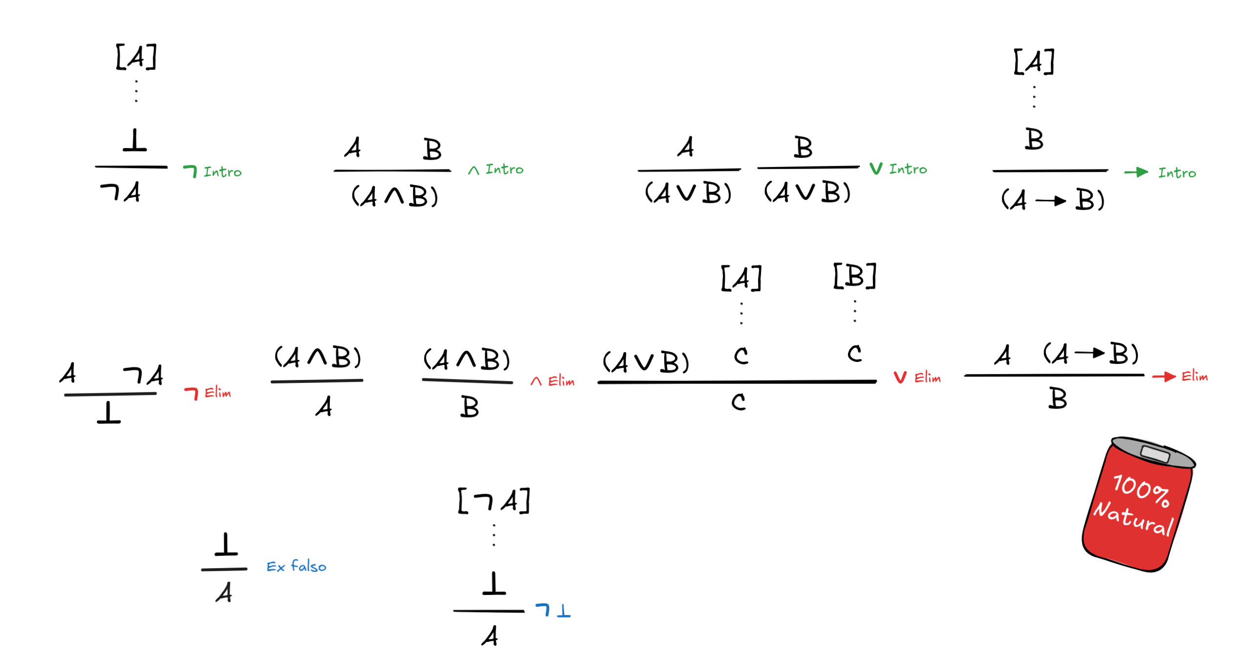
Some of these rules require a bit more explanation. Take the rule Introduction, for example. This rule has corner brackets around its premise, [A]. What this means is that the assumption A is discharged in the application of Introduction—after the application of the rule, A no longer counts among the assumptions of the proof.

Applying this rule, we can for example reason as follows:

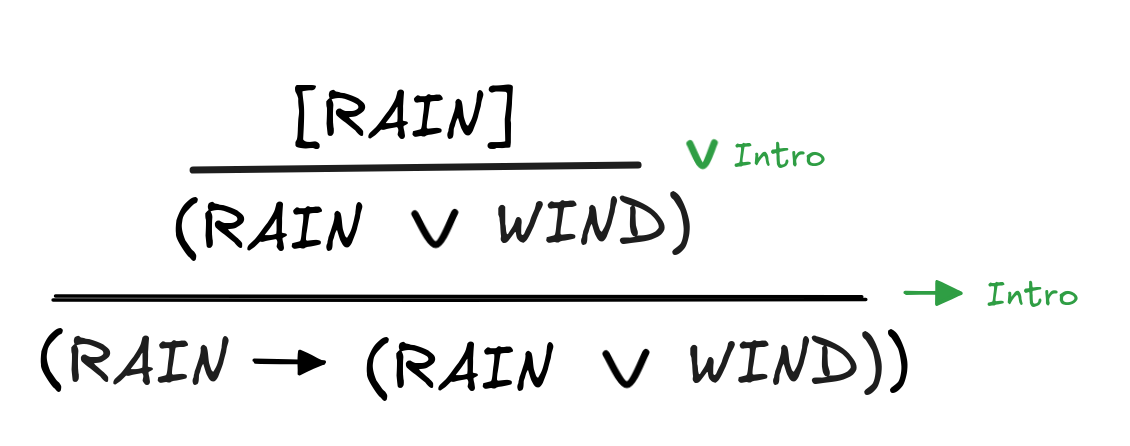
We assume that it rains. From this we infer that it’s rainy or windy. So, even without the assumption, we know that if it rains, then it’s rainy or windy. In other words, what this derivation establishes is that (RAIN (RAIN WIND)) can be derived without any assumptions:

(RAIN (RAIN WIND))

In rules like Elim, this hypothetical reasoning with discharging assumptions is taken to the next level. This rule captures case-by-case reasoning, which we can use, for example, to show the validity of our previous example for disjunctive syllogism in natural deduction:

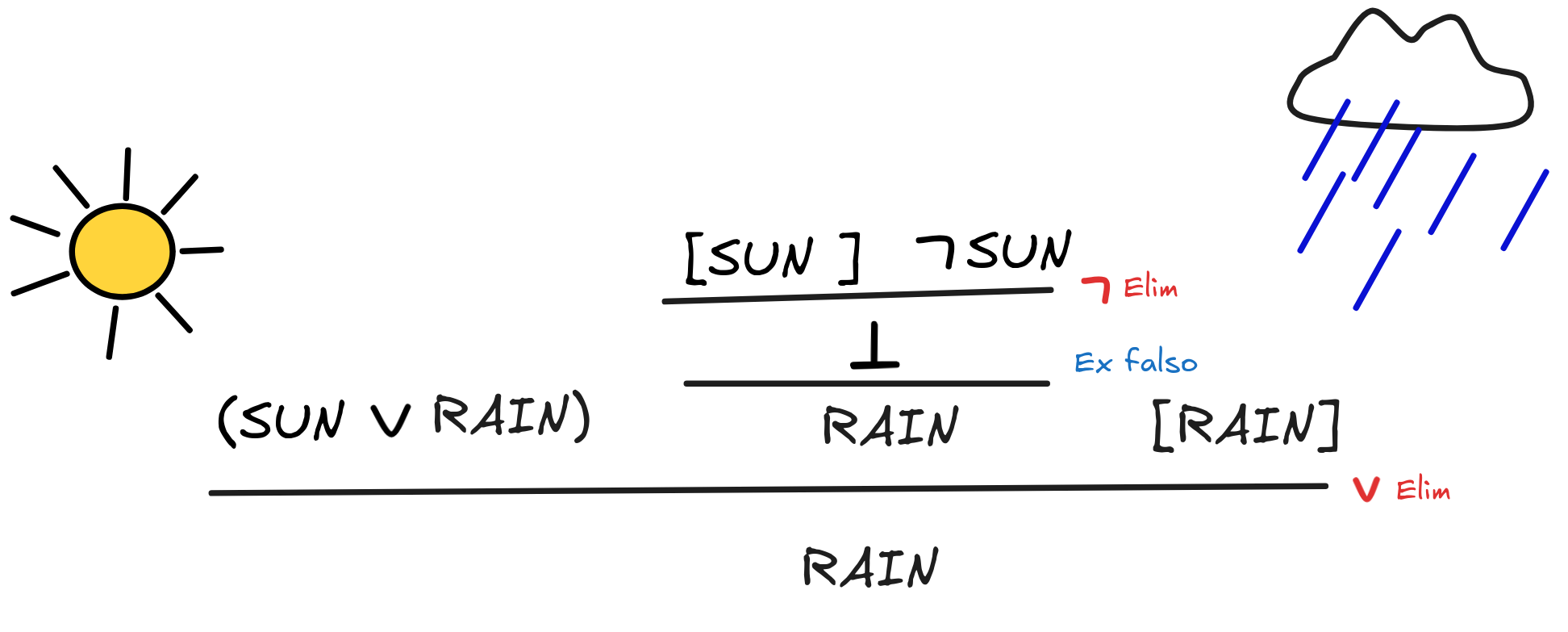
What’s going on here is that we assume both (SUN RAIN) and SUN. We know that the disjunction means that there are two possible cases, either SUN or RAIN, so we think both through. We assume sun in addition to our other assumptions, and note that we got a contradiction with our other assumption SUN, which yields . From this, we can use the principle of explosion, which we’ve captured in the rule Ex falso to infer that RAINS. That leaves only the other possible case. If we assume that it rains, it rains, so we can discharge the assumption directly. We infer that it must be raining. This proof shows that

(SUN RAIN), SUN RAIN

The rules Ex falso and deserve special attention since they capture logical laws that are only valid in very specific logical contexts or systems. The principle of explosion, which we’ve just used to proof disjunctive syllogism, for example, is valid in Boolean logic. Here, we can derive the falsum from any contradiction, like SUN and SUN. This is because SUN cannot both be true and false at the same time. But that means that if we assume that it is, we get and “anything goes”, so if both SUN and SUN, then RAIN.

Or think about it the other way around. The only way for the inference from SUN and SUN to RAIN be invalid is for both SUN and SUN to be 1, while RAIN is 0. But in Boolean logic that’s excluded. So the inference must be valid.—If we move to a paraconsistent logic, however, where statements can be both true and false at the same time, things change. Such logics are very important when combining potentially contradictory information from different databases, but that’s a story for later on.

The case of is equally fraught with logical and philosophical issues, but suffice it to say here, that it is required to derive RAIN RAIN. This principle fails, for example, in intuistionistic logic, which is of paramount importance in the foundations of computation. We won’t be able to go into the full details here, but we’ll see that these special rules play an important role, for example, when we move to proof assistants.

There’s one more stumbling block for natural deduction, which is worth mentioning. Though perhaps strange, the following is a valid derivation in natural deduction:

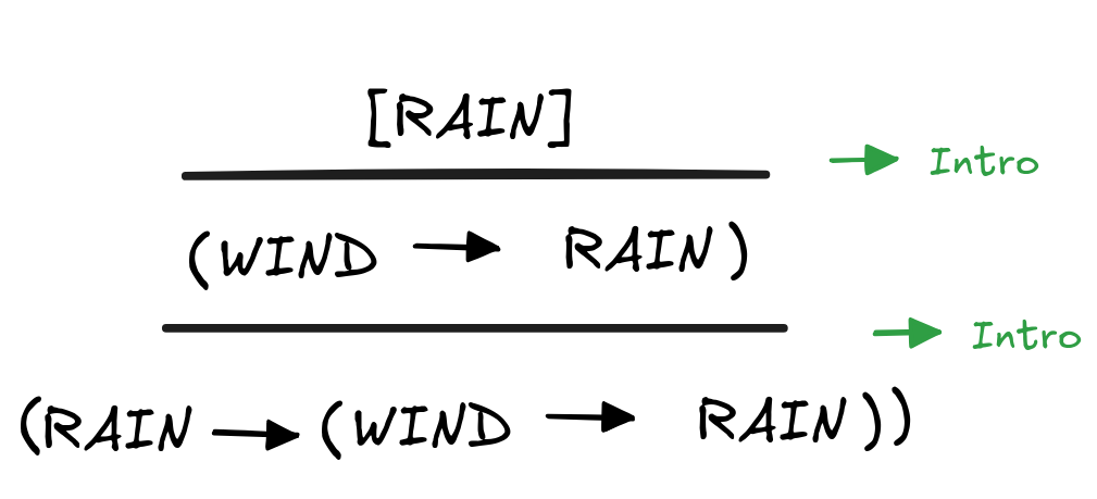
What’s going on here is that in the first application of Intro, the assumption WIND is discharged even though it’s not written down anywhere. This is called vacuous discharge and without it, we couldn’t prove laws like the one from the derivation, which is one of Hilbert’s axioms. The assumption RAIN, then, can be discharged as normal.

It’s also worth pointing out that are actually many different notational system for natural deduction: we use the Genzten-Prawitz-style, but there are also Fitch-notation, Suppes-Lemmon notation, and many others.

As we said, natural deduction attempts to model the most basic, small-step inferences we make in natural language reasoning. At the same time, as any math student can attest, making good small-step inferences is hard work—even in natural language. So, it should come as no surprise that learning to make correct natural deduction inferences for is hard work. And unfortunately, there’s no shortcut around just trying one’s hand at this. Luckily, there are tools that allow us to check our own work: these are the proof assistants we’ve mentioned before and will talk about next.

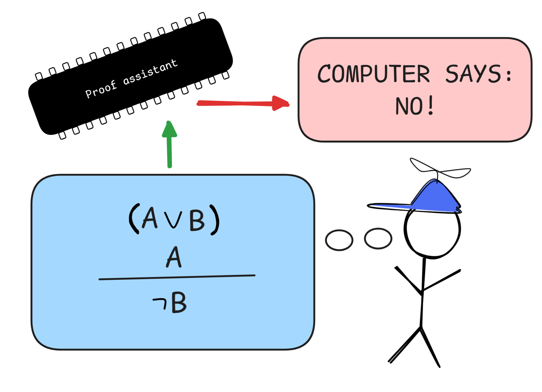
Proof assistants: Lean

A proof assistant is a piece of software that helps develop logical proofs in a kind of human-machine collaboration. The idea is that to interact with a proof assistant, we write down our proofs in a specialized formal language, which the proof assistant can easily parse and then check for formal reasoning mistakes—that is, check whether we’ve applied the rules and conditions for logical proofs correctly. This is a paradigm case of intelligence amplification (IA), where we “outsource” the verification of our arguments to a specialized computer program.

What might seem like a very dry and nitpicky activity at first, turns out to be an incredibly helpful and powerful logical tool for research in disciplines that rely heavily on the correctness of mathematical arguments, such as pure and applied math, physics, economics, and others. While trained mathematicians are experts at giving logical proofs, mistakes do happen. Mathematicians are human after all. To find these mistakes is the aim of peer review, but the more advanced the work, the fewer peers there are. When it comes to cutting-edge research mathematics, it’s not at all uncommon that there are only a handful of people in the world who fully grasp the arguments of a research paper.

As a result, there are often only few people who can spot mistakes. And these are typically people that do similar work as the author, and so are more likely to “think just like them”—and as a consequence make the same kind of mistakes. This is an in principle problem when we’re working with fallible reviewers in highly-specialized disciplines like mathematics. Proof assistants can help mitigate these issues. In fact, there are several high-profile cases, where proof assistants both helped spot and fix errors in the work of Fields medalists and other high-profile mathematicians.

Terence Tao has recently argued that the added certainty that a verification by a proof assistant adds is a great boon for mathematical collaboration, since you no longer need to carefully check all the proofs of your potential collaborators—the computer does that for you. This opens up the possibility of new kinds of collaboration.

At the same time, way that proof assistants interface with natural language proofs is very adaptable to the way that LLMs treat texts. This opens up the possibility of GenAI-technologies, like ChatGPT, Claude, Gemini, and others, using proof assistants to formulate and verify their reasoning. The potential for applications of this observation in machine learning and practice are endless. What we see in practice already is that AI-tools like GitHub Copilot can complete some simple mathematical arguments while they are being typed in LaTeX source code by an author.

There are many proof assistants out there, such as Agda, Isabelle/HOL, and Coq. But in this course we’ll be working with the Lean proof assistant, which has gotten a lot of traction in the mathematical community recently. This is in part because of the ease of working with Lean, and in part because of the incredible community surrounding the proof assistant. There is a lot of documentation, examples, and huge libraries, like mathlib, which contains proofs for a vast amount of important mathematical theorems, fully formalized and verified in Lean.

Lean is, in effect, a programming language. To verify a proof, you essentially write a computer program in the Lean programming language, which when run will return errors if there are mistakes in the proof. The details are, of course, much bit more complicated, but for our purposes, this picture is enough for now.

Lean-code can be compiled into a stand-alone program or it can be run directly in your text-editor by an interpreter. Using an interpreter means that we can write a proof-as-code and get live feedback on our work while writing it. Amazing! Of course, you can install lean on your own computer, but for your first steps in the language, you can also use the lean playground, which runs directly in your browser.

The Lean language is based on Thierry Coquand’s calculus of constructions (COC). It is a full-fledged functional programming language. And of course, we won’t be able to give a comprehensive tutorial here. But what we can do is look at the way we can verify basic logical proofs in propositional logic in Lean, live in your browser.

Here is a verification of our running example in Lean:

1
2
3
4
5
6
7
8
9

variable (RAIN WIND COLD HEATING: Prop)

example (rain : RAIN)
        (if_rain_or_wind_then_cold : (RAIN ∨ WIND) → COLD)
        (if_cold_then_heating : COLD → HEATING) :
    HEATING := by
  apply if_cold_then_heating
  apply if_rain_or_wind_then_cold
  apply Or.inl rain

Click this link to run this code in your browser. As you can see, no error messages are returned, the proof is correct.

Let’s unfold what’s going on here.

In the first line

1

 variable (RAIN WIND COLD HEATING: Prop)

we declare the variables RAIN, WIND, COLD, HEATING to be of type Prop. The background theory of Lean is a powerful system of types, the aforementioned COC, but all we need to know here is that the syntax here means that RAIN, WIND, COLD, HEATING are Props and Prop is Lean’s type for propositions, which can be either true or false.

Next, we declare that we’re trying to prove an example:

3
4
5
6

example (rain : RAIN)
        (if_rain_or_wind_then_cold : (RAIN ∨ WIND) → COLD)
        (if_cold_then_heating : COLD → HEATING) :
    HEATING := by

This declaration has itself a complex structure. It begins with the straight-forward keyword example to indicate that we’re dealing with an example. This immediately followed by a sequence of additional declarations:

  (rain : RAIN) 
  (if_rain_or_wind_then_cold : (RAIN ∨ WIND) → COLD) 
  (if_cold_then_heating : COLD → HEATING)

To understand what’s going on here, we need to talk about how Lean works “under the hood”. What we’re saying here is, essentially: suppose that rain is a proof of the proposition RAIN, if_rain_or_wind_then_cold is a proof of (RAIN WIND) COLD, and if_cold_then_heating is a proof of COLD HEATING. Our aim is to show how we can transform these proofs into a proof of HEATING, this is what we declare by following this declaration by “: HEATING”.

One of the ideas underlying Lean is that saying that a proposition is true and that there exists a proof of it are, in many contexts, exchangeable. So, basically, by “witnessing” each of our propositional variables by a proof (which we indicate in lowercase), we’re assuming that these propositions are true. And what our ultimate inference does is to convert these proofs into a proof of HEATING—which means we show that HEATING is true if the premises are. In other words, we show that our inference is valid.

What follows next is the formal proof in Lean. It follows our declared goal HEATING:

6
7
8
9

    HEATING := by
  apply if_cold_then_heating
  apply if_rain_or_wind_then_cold
  apply Or.inl rain

The := here indicates that a proof begins. The by indicates that we’re using what’s known as tactic mode. We already mentioned that in Lean, we’re basically converting proofs of assumptions into proofs of our conclusion. This works by means of proof constructions (whence the name “Calculus of Constructions”), which we can write down in different ways. We can directly apply the constructions of COC, leading to expressions in what’s known as typed lambda caclulus. These expressions are the formal foundation of what’s going on “under the hood”, but they are very difficult to understand for humans.

Luckily, Lean (like many other proof assistants) has the tactic mode. This is essentially a more human-readable way of expressing formal arguments. We indicate that we want to use this mode by using the keyword by.

What comes next is the actual proof. It’s best to read that proof from bottom to the top. The line

9

  apply Or.inl rain

takes the proof of RAIN and applies to it (what’s effectively) the natural deduction rule Intro. That is, this line represents the natural deduction inference:

Note that we don’t need to tell Lean that we want the other disjunct to be WIND. It will figure this out by itself using automated reasoning techniques, which we’ll discuss later in the course.

The next line working backwards is:

8

  apply if_rain_or_wind_then_cold

Note that the apply keyword, which took 2 arguments in line 9, only seems to have one argument here. We’re applying the proof if_rain_or_wind_then_cold for (RAIN WIND) COLD. But to what?

The answer is that we apply it to the next line, that is line no 9. The expression here is parsed just like the following one-liner:

  apply if_rain_or_wind_then_cold (apply Or.inl rain)

That is Lean recursively applies the proof for (RAIN WIND) COLD to the result of applying the Intro-rule to the proof for RAIN.

But what does it mean to apply a proof for (RAIN WIND) COLD to a proof for (RAIN WIND) COLD? The answer is rather obvious: apply MP to infer COLD—which is precisely what Lean does here. That is, at this point, we’ve constructed in Lean the following natural deduction proof:

Now it should be clear how the proof finishes. The last apply takes the proof for COLD HEATING to our proof for COLD. That is, reading the lines

7
8
9

  apply if_cold_then_heating
  apply if_rain_or_wind_then_cold
  apply Or.inl rain

as

  apply if_cold_then_heating (apply if_rain_or_wind_then_cold (apply Or.inl rain))

we’ve constructed our full natural deduction proof:

Lean is happy. It says that all goals are satisfied and doesn’t return an error. We’ve verified our natural deduction inference using Lean 🎉 (Note: This emoji is used by many Lean interpreters to indicate success. It’s also a party popper.)

Running through the example, we’ve uncovered one of the most fundamental principles of the theory of computation, which underlies the way Lean verifies proofs: the so-called Curry-Howard correspondence. Simply put, the Curry-Howard correspondence states that there’s an equivalence between computer programs and mathematical proofs. The way this shows up here is that the Lean constructions, which are essentially (and very practically) computer programs correspond in a one-to-one fashion to natural deduction inference rules. This correspondence allows us to go back and forth between natural deduction proofs and Lean programs and it’s the very foundation of how Lean ultimately works.

The correspondence is most clearly visible in the case of conjunctions and disjunctions. For each the corresponding introduction and elimination rules, there are corresponding Lean tactics:

• -Intro corresponds to And.intro, which applied to the proofs of two propositions yields a proof of their conjunction.
• -Elim corresponds to the two tactics And.left and And.right, which when applied to proofs of a conjunction yield proofs of the left or right conjunct respectively.
• -Intro correspond to Or.inl and Or.inr, which when applied to proofs of a proposition yield the disjunction with some other formula on the left or on the right (Lean figures out which one you mean).
• -Elim corresponds Or.elim, which when applied to two proofs of a given conclusion from each of two disjuncts, gives a proof of that conclusion from the disjunction itself.

Here’s a simple example to illustrate how this works for -Intro/Elim and -Intro:

1
2
3
4
5
6
7
8

(variable RAIN WIND SUN : Prop)

example (rain_and_wind : RAIN ∧ WIND) : (RAIN ∨ SUN) ∧ (WIND ∨ SUN) := by 
  apply And.Intro
  apply Or.intro 
  apply And.left rain_and_wind
  apply Or.intro
  apply And.right rain_and_wind

Click this link to run this code in your browser.

This code verifies the following natural deduction proof:

(RAIN WIND) (RAIN SUN) (WIND SUN)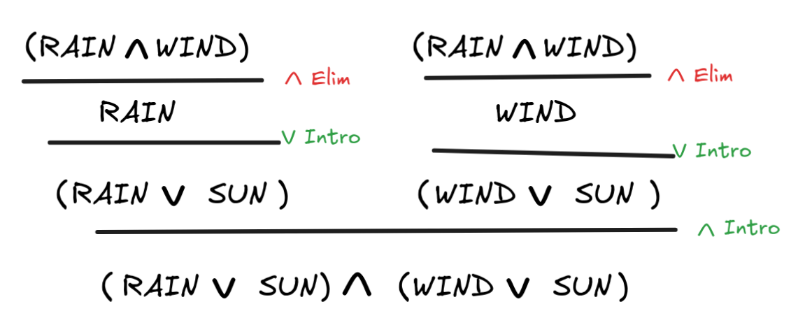

Before we can talk about -Elim, we need to talk about the conditional. We’ve actually already discussed how -Elim works in Lean: if we have a proof of a conditional, we can directly apply it to a proof of its antecedent to obtain a proof of the consequent. So, how do we do -Intros?

Remember that -Intro works by hypothetical reasoning: to prove A B, we derive B from the assumption that A, which we discharge in the process. In Lean, we introduce an assumption like this using the intro tactic. Here’s how this works in practice:

1
2
3
4
5
6

(variable RAIN WIND: Prop)

example : RAIN → (RAIN ∨ WIND) := by 
  intro rain
  apply Or.inl
  exact rain

Click this link to run this code in your browser.

This is the Lean verification of our earlier natural deduction proof for RAIN (RAIN WIND):

The intro-tactic introduces a new hypothesis into the space, which we give the name rain. Lean figures out by itself that this is supposed to be the hypothesis for the if part of the conditional RAIN (RAIN WIND)—i.e. for RAIN—since that’s what we need to prove at this point.

Note that in the last line we write exact rain, rather than just rain, which would also have been fine. The tactic exact is “ syntactic sugar” for the apply-tactic, which you’re supposed to use when your proof is complete. It doesn’t do anything else than apply or not writing anything, but it will fail give more transparent error messages if proof doesn’t quite work—and in this way, exact fosters code Lean practice.

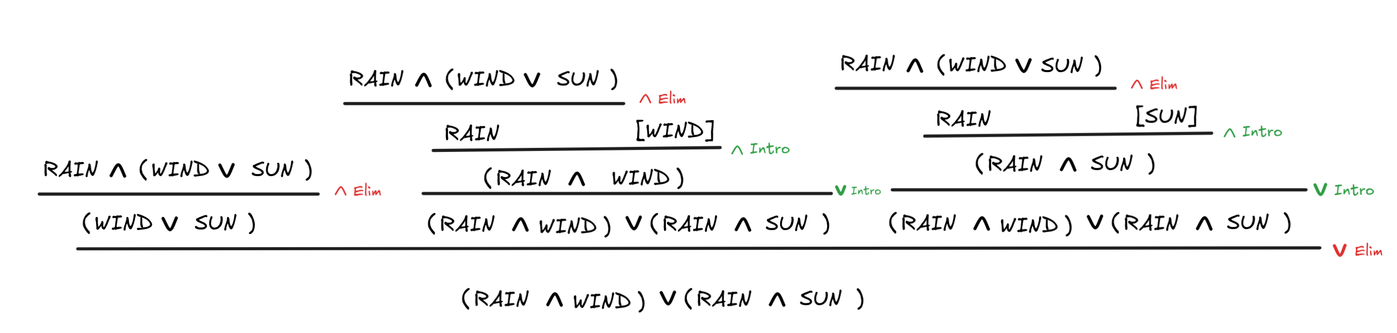
With this in hand, we can move to Or.elim. To illustrate, let’s look at a more complex example. Let’s verify the following in Lean:

RAIN (WIND SUN) ((RAIN WIND) (RAIN SUN))

Here is the Lean code:

 1
 2
 3
 4
 5
 6
 7
 8
 9
10
11
12
13
14
15

variable (RAIN WIND SUN : Prop)

example : RAIN ∧ (WIND ∨ SUN) → (RAIN ∧ WIND) ∨ (RAIN ∧ SUN) := by
  intro rain_and_wind_or_sun
  apply Or.elim (And.right rain_and_wind_or_sun)
  · intro wind
    apply Or.inl
    apply And.intro
    · exact And.left rain_and_wind_or_sun
    · exact wind
  · intro sun
    apply Or.inr
    apply And.intro
    · exact And.left rain_and_wind_or_sun
    · exact sun

Click this link to run this code in your browser.

This code corresponds to the following derivation in natural deduction:

There are a few things going on here. As we’ve discussed before, the Lean can work out itself that the following line

4

  intro rain_and_wind_or_sun

introduces the assumption that RAIN (WIND SUN). Lean “knows” this because we’re trying to prove the conditional:

RAIN (WIND SUN) ((RAIN WIND) (RAIN SUN))

and the assumption we have to make for this is that RAIN (WIND SUN).

Correspondingly, when we apply And.right to this assumption, this gives us a proof of the disjunction (WIND SUN) in

5

  apply Or.elim (And.right rain_and_wind_or_sun)

To this disjunction, we apply the rule OR.elim. But the tactic needs to more arguments, which is what’s provided next:

 6
 7
 8
 9
10
11
12
13
14
15

  · intro wind
    apply Or.inl
    apply And.intro
    · exact And.left rain_and_wind_or_sun
    · exact wind
  · intro sun
    apply Or.inr
    apply And.intro
    · exact And.left rain_and_wind_or_sun
    · exact sun

The bullet points · are, again, “syntactic sugar” (you can typeset them by typing “\.” in the online text-editor). They structure the sub-proof in such a way that we can more easily see what’s going on—which is that we have two proofs, one from WIND and one from SUN both ending in ((RAIN WIND) (RAIN SUN)), as desired.

Note that also here, Lean can work out by itself that wind is a proof of WIND and sun a proof of SUN. In fact, we don’t need to use the mnemonic names here, the following code provides the exact same result:

 1
 2
 3
 4
 5
 6
 7
 8
 9
10
11
12
13
14
15

variable (RAIN WIND SUN : Prop)

example : RAIN ∧ (WIND ∨ SUN) → (RAIN ∧ WIND) ∨ (RAIN ∧ SUN) := by
  intro h
  apply Or.elim (And.right h)
  · intro i
    apply Or.inl
    apply And.intro
    · exact And.left h
    · exact i
  · intro j
    apply Or.inr
    apply And.intro
    · exact And.left h
    · exact j

Click this link to run this code in your browser.

The structure of the derivation is enough for Lean to work out what h,i, and j stand for.

So far, we’ve been dealing with example kind of declarations. But once we start building a more extensive library of Lean code, we want to start naming our results. The standard way of doing this is using the theorem declaration followed by a name. The following code gives an example:

1
2
3
4
5
6
7

theorem absorption_right_to_left (A B : Prop): A ∨ (A ∧ B) → A := by
  intro a_or_a_and_b
  apply Or.elim a_or_a_and_b
  · intro a
    exact a
  · intro a_and_b
    apply And.left a_and_b

Click this link to run this code in your browser.

Note that in this proof we also declare our variables inside the name declaration, which also works with example-style declarations. And we used non-mnemonic variables A and B, which is more common when you’re proving general logical laws.

Once we have a name for a theorem, we can use it in later proofs (which, of course, need to load the earlier proof as well). That is, if we have the previous code, we can simply apply absorption_right_to_left to a proof of A (A B) to obtain a proof of A.

This gives you an idea of how to verify proofs in Boolean propositional logic involving , , and using tactics-based Lean code. Of course, Lean is much, much more powerful than that: it can verify logical proofs from even the most cutting-edge areas of mathematics and physics with relative ease—this is part of its appeal to mathematicians!

You’ll learn more advanced Lean techniques later in this course, but before we move on to other logical systems, we should discuss how the negation operator works in Lean.

For this, let’s inspect the natural deduction rules for :

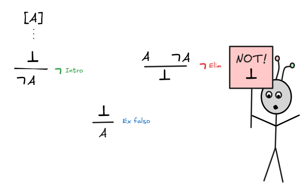
The thing to note here is that A behaves exactly like A , where is the special falsum constant. Lean takes this to be the defining feature of negation, which is an idea that traces back to Lean’s intuitionistic-roots, which we don’t have time to look into now.

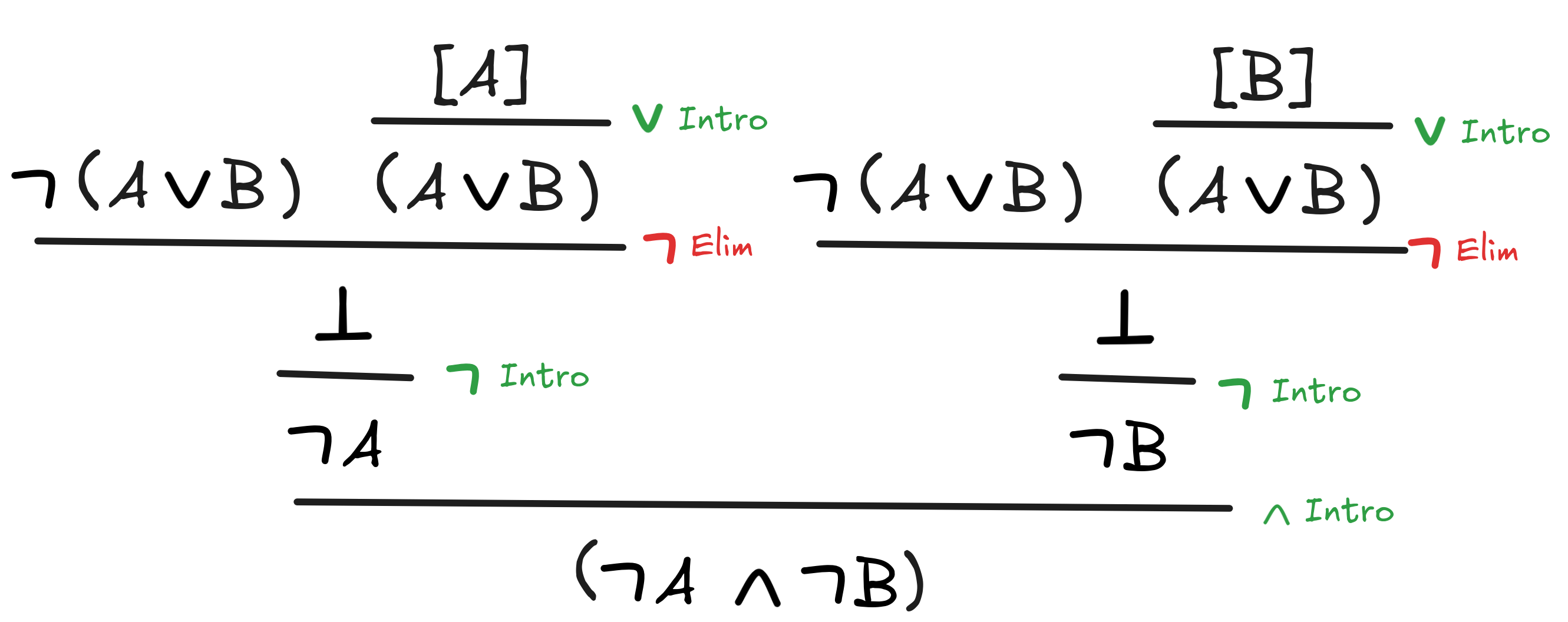
This means that we can apply formulas of the form A to formulas of the form A to obtain a proof of , and if we can derive from a formula A, this gives us a proof of A. Here is an example that illustrates both ideas at the same time:

 1
 2
 3
 4
 5
 6
 7
 8
 9
10
11

theorem de_morgan_one_ltr (A B : Prop): ¬(A ∨ B) → (¬A ∧ ¬ B) := by
   intro not_a_or_b
   apply And.intro
   · intro a
     apply not_a_or_b
     apply Or.inl
     exact a
   · intro b
     apply not_a_or_b
     apply Or.inr
     exact b

Click this link to run this code in your browser.

Under the ideas just outlined, this code corresponds to the following natural deduction proof:

Note that in our Lean derivation, we didn’t need to write out , but if you ever have to, it works by writing False. That is, you can write “A → False” instead of “¬A” and say the same thing.

The principle Ex falso, which states that you can derive any consequence from a contradiction has the equivalent Lean tactic False.elim, which you can also refer to by absurd. So, we can prove the law:

1
2
3
4
5

theorem ex_falso_quodlibet (A C : Prop) : (A ∧ ¬ A) → C := by
  intro a_and_neg_a
  apply False.elim
  apply And.right a_and_neg_a
  exact And.left a_and_neg_a

Click this link to run this code in your browser.

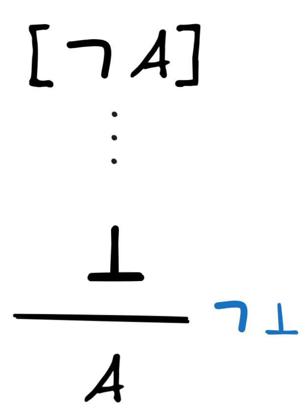
What’s left is to discuss the rule , which is peculiar in natural deduction, as in Lean:

This rule is not standardly available in Lean. This again has to do with Lean’s roots in intuitionistic logic, where the rule fails. But we can load the rule by the line open Classical. The rule is needed, for example, to derive the law of double negation elimination:

1
2
3
4
5
6

open Classical

theorem double_negation_elim (A : Prop) : ¬¬A → A := by
  intro not_not_a
  apply byContradiction
  apply not_not_a

Click this link to run this code in your browser.

What’s going on here is that by the line open Classical, we make the new tactic byContradiction available, which allows us to derive A from a proof of ⊥ from the assumption that ¬A. This is precisely what’s going on here:

4
5
6

  intro not_not_a
  apply byContradiction
  apply not_not_a

The tactic byContradiction introduces the hypothesis not_a, which is a proof of ¬A. We apply our previous assumption not_not_a to this to obtain False via MP, which is enough to infer A according to the idea underlying .

This concludes our teaser of Lean for proof verification in classical Boolean logic. This is just the very beginning of a huge field of active AI research, which has the potential to change the way we use mathematics in our research. There are attempts to use traditional ATP-techniques “proof search” to automate the search for proofs via tactics like exact?, which searches the mathlib-library for any theorem that fits all the open assumptions we currently have. This could help researchers find results even if they’ve never heard of them.

At the same time, Lean is playground for GenAI techniques, which in 2024 helped researchers at Google’s DeepMind research group develop an AI-system that achieved silver-medal standard at IMO problems.

Further readings

An excellent introduction to structural proof theory is Sara Negri and Jan van Plato’s Structural Proof Theory. CUP 2010.

If you want to learn more about Lean and its use for proof verification, a great place to start is Theorem Proving in Lean 4 by Jeremy Avigad, Leonardo de Moura, Soonho Kong, Sebastian Ullrich, and contributions from the broader Lean Community.

A great “playground” is the natural number game. In general, the Lean Game Server contains an awesome collection of gamified introductions to Lean.

You can find an amazing talk about how AI can influence science and mathematics, in part using proof systems under https://www.youtube.com/watch?v=_sTDSO74D8Q.