Boolean satisfiability

---

We’ve seen that Boolean logic is at the heart of computation and deductive reasoning. But when it comes to automated reasoning, our approach has so-far been limited to pre-programmed circuits, like the logic gates and adders we’ve discussed. While these circuits are great at carrying out specific deductive reasoning tasks, like adding two numbers or calculating truth-values, they are not very flexible. Each circuit carries out one specific task.

But in AI, we don’t only want to implement specific inference patters using specific cirucits, like adding two bits using an adder circuit or inferring (A B) from A and B using AND. We want to implement deductive reasoning in general.

We did already discuss an implementation of deductive inference in Boolean logic, but the approach still required human intervention. To determine whether a certain inference is valid, like whether (SUN RAIN), SUN RAIN, we manually needed to check all possible valuations to see whether there is one that makes the premises true and the conclusion false.

Satisfiability solving is a powerful approach to automated reasoning using Boolean logic, which is popular in research and industry alike. The observation that motivates the approach is that we can reduce the question whether a given inference is valid to the question whether certain truth-value assignment is possible. SAT-solving algorithms are instructions for systematically—and ideally efficiently—testing for the existence of specific truth-value assignments.

The applications of this powerful logical method for AI reasoning range from formal hardware verification to automated reasoning in propositional languages and beyond.

At the end of this chapter you’ll be able to:

• define the SAT problem for Boolean formulas and explain its relevance to logic and artificial reasoning

• apply the truth-table method for satisfiability checking

• convert formulas into disjunctive and conjunctive normal form

• apply the resolution algorithm and explain its advantages over the truth-table method

SAT

---

There are both algebraic and logical ways of thinking about the Boolean satisfiability problem or SAT.

We’ll start thinking algebraically, where SAT asks whether for a given Boolean expression, like:

whether there exists an assignment of values to X and Y, such that the expression evaluates to 1. In this case, the answer is yes, since for X = 1 and Y = 1, we get the calculation:

We say that the expression is satisfiable.

If we take the following Boolean expression, instead:

we find that no matter the value for X, the formula evaluates to 0:

• If X = 1, then 1 AND NOT (1 OR 1) = 1 AND NOT 1 = 1 AND 0 = 0

• If X = 0, then 0 AND NOT (0 OR 1) = 0 AND NOT 1 = 0 AND 0 = 0

This Boolean expression is unsatisfiable.

The idea of satisfiability can be extended to sets of Boolean expressions in a natural way: we say that a set of Boolean expressions is satisfiable just in case there is an assignment to its variables that makes all the members of the set true.

Here’s an example of a satisfiable set of Boolean expressions:

This is because for the values X = 0, Y = 0, Z = 1, we get:

• (NOT X) AND (Y OR Z) = (NOT 0) AND (0 OR 1) = 1 AND 1 = 1

• X OR (NOT Y) = 0 OR (NOT 0) = 0 OR 1 = 1

• Z OR (NOT Z) = 1 OR (NOT 1) = 1 OR 0 = 1

Here’s an example of an unsatisfiable set:

No matter what the value of X, at least one formula evaluates to 0:

• If X = 1, then X OR 0 = 1 OR 0 = 1, but (NOT X) AND 1 = (NOT 1) AND 1 = 0 AND 1 = 0.

• If X = 0, then (NOT X) AND 1 = (NOT 0) AND 1 = 1 AND 1 = 1, but X OR 0 = 0 OR 0 = 0.

It turns out that many important problems can be reduced to questions of satisfiability. One important example is (formal) hardware verification. To discuss the idea in a simplified example, let’s go back to relay logic.

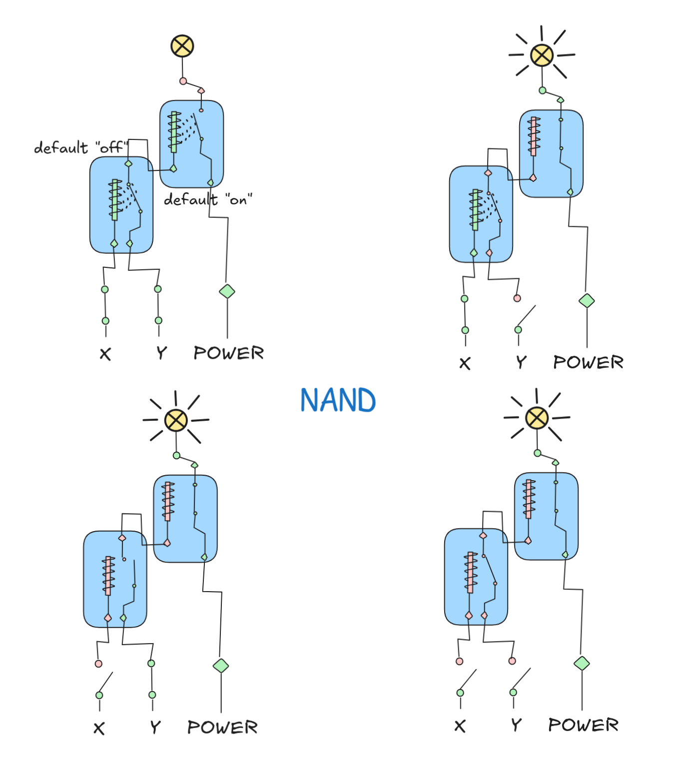
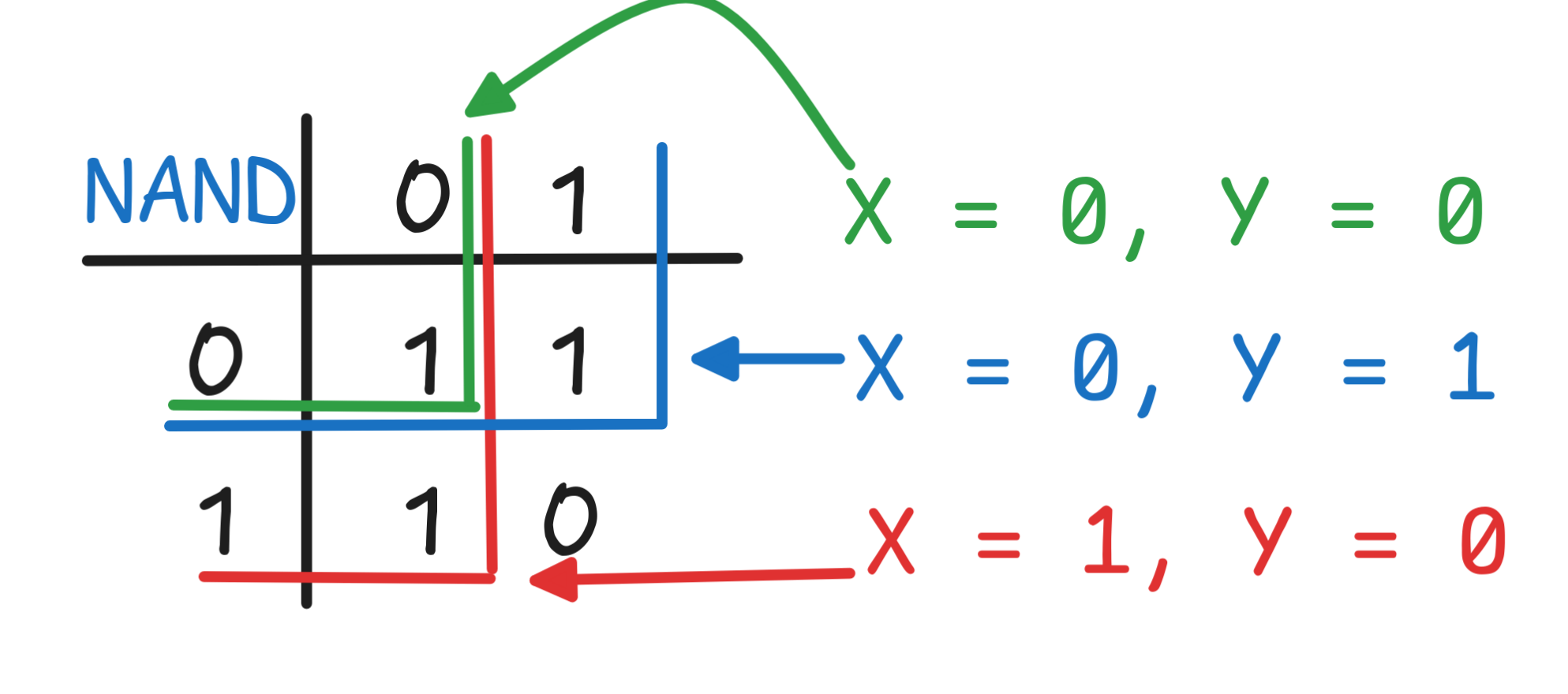
We implemented different truth-functions using relays. One example (from the exercises) is the NAND function, which has the following function table:

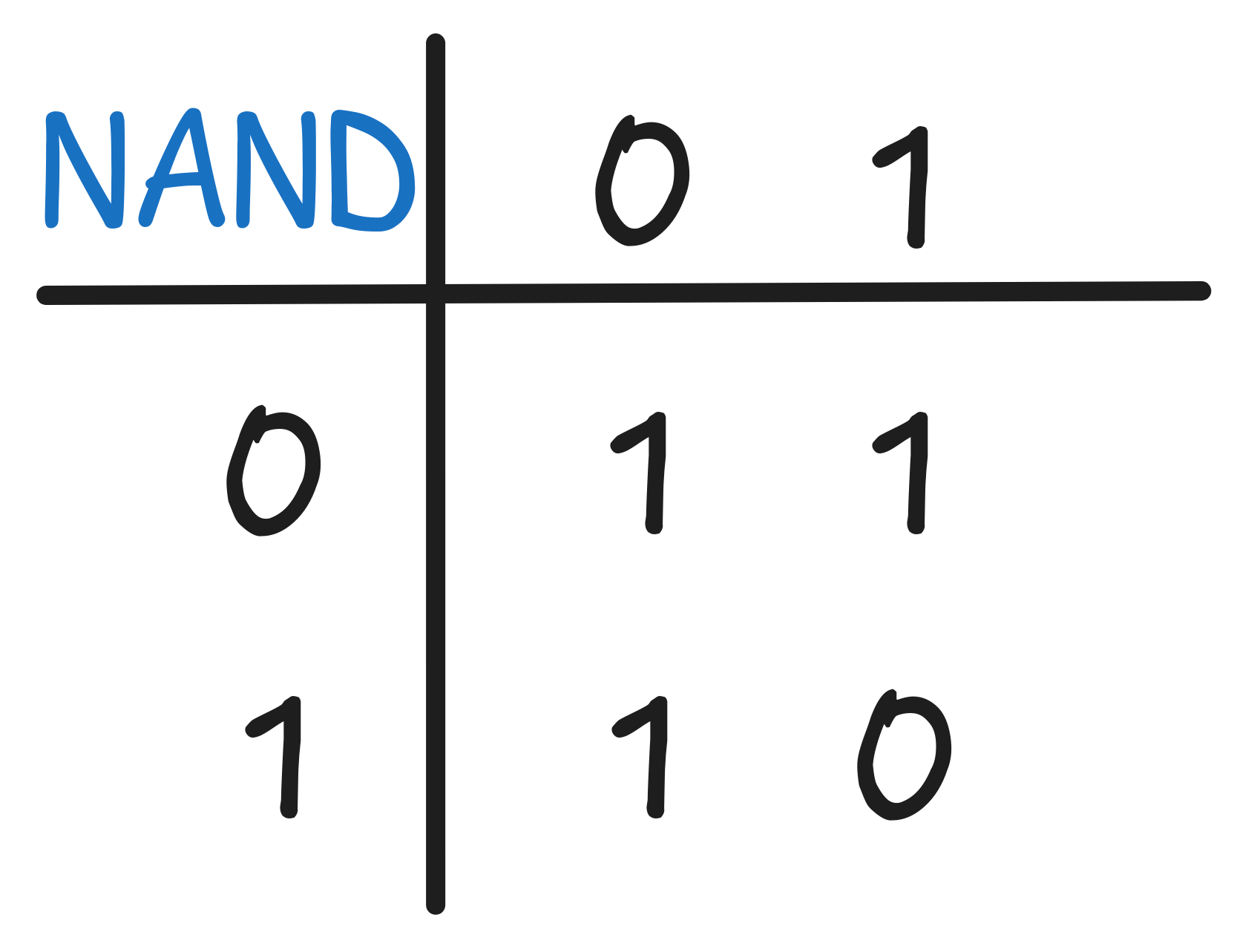
We can implement this with the following relay circuit (spoiler alert, if you didn’t do the exercises yet 😉):

To check that this implementation is according to the specification given by the function table, we need to go through all the possible inputs and check that the circuit gives the same outputs for the same inputs as the table says.

This is a bit tedious, but doable for smaller circuits with few inputs and outputs and rather simple specifications, like our NAND table. But in practice, circuits get much, much larger. A modern CPU, for example, contains in the order of hundreds of millions to billions of logic circuits, which implement a specification like the X86 instruction set or ARM instructions. Here, we simply cannot go through all the possible input configurations and check whether the outputs are correct. We need a more efficient method.

SAT-solving provides one popular approach for this, which is, in effect, industry standard. We cannot discuss the full details, but we can illustrate the idea using our NAND circuit.

For the approach, we need to translate both our specification (the NAND table) and our circuit into Boolean expressions. For the circuit, this is rather straight-forward, once we realize that a default “off” relay is essentially a Boolean AND and a default “on” relay is a Boolean NOT. Inspecting our circuit, we see that we just chain the default “off” and default “on” relays with the inputs. This means that the Boolean expression that corresponds to our circuit is:

This is the origin of the term “NAND”, by the way: NOT applied to AND … NAND.

Formalizing the specification is a bit more involved, but it turns out that there’s a powerful method for expressing truth-functional tables using the Boolean operators NOT, AND, and OR.

If you have a binary truth-function, like NAND, the expression that we’ll generate by our method involves two variables X and Y. The first, X, represents the first input (the first column of the function table), and Y represents the second input. We write a Boolean expression in X and Y, which represents the output. For this, we first identify all the input configurations, which give output 1, which in this case are:

Now, each of these configurations will turn into a clause in our Boolean representation, which joins these clauses using OR. To obtain these clauses, we represent the input configuration X = 1 by writing simply X, and the input configuration X = 0 by writing NOT X. Then we do likewise for Y and combine the corresponding representations for X and Y using AND. This gives us:

• for the first configuration, the clause: (NOT X) AND (NOT Y)

• for the second configuration, the clause: (NOT X) AND Y

• for the third configuration, the clause: X AND (NOT Y)

The final Boolean expression joins the clauses using OR, giving us:

This method is guaranteed to generate a Boolean expression that describes the truth-table it was generated from. In fact, we can use this method to prove that every truth-function can be represented using NOT, AND, and OR, but that’s for another time. The resulting formula is also called the full or maximal Disjunctive Normal Form (DNF) representation of the truth-table—these kind of normal forms we’ll return to later.

Now, we’ve got two formulas:

• a specification: ((NOT X) AND (NOT Y)) OR ((NOT X) AND Y) OR (X AND (NOT Y))

• and a circuit representation: NOT (X AND Y)

The question is whether the circuit implements the specification, that is whether the two expressions always have evaluate to the same truth-values. That is:

• If the specification evaluates to 1, does the representation evaluate to 1?

• If the representation evaluates to 1, does the specification evaluate to 1 as well.

We can, of course, check this by going through the possible values for X and Y again, but the point here is that we can reduce this problem to a SAT problem.

For this, the trick is to check whether it’s possible that the two expression evaluate to different values. That is, is it possible that:

• The specification evaluates to 1 and the representation to 0.

• The representation evaluates to 1 and the specification to 0.

The last ingredient is to note that an expression evaluates to 0 just in case NOT applied to the expression evaluates to 1—this is just the function table for NOT. But then, we can reduce our question to the SAT problem for the following two sets:

In our example, the question is whether any of the following two sets is satisfiable:

If any of the two sets is satisfiable, our circuit implementation does not follow the specification. If neither of them is satisfiable, our circuit is correct.—We’ve reduced the verification of the circuit to a SAT problem.

While it may look like we’ve made things worse—the Boolean expressions we wrote down are not per se easier to understand than the initial problem—we’ve actually massively improved our situation. We’ve figured out a way of mechanically translate the question whether our circuit functions according to specification into a SAT-problem. And as we’ll see, the SAT problem itself allows for algorithmic approaches. This is the foundation for automated circuit verification. Similar ideas are used for software verification

In industry practice, the setup is, of course, much more complicated. There we’re dealing with huge circuits and highly complex specifications, much more complicated than our simple function table and relay circuit. To deal with this, we use advanced technologies, like hardware specification languages and dedicated SAT solvers. But the ultimate ideas are still the same.

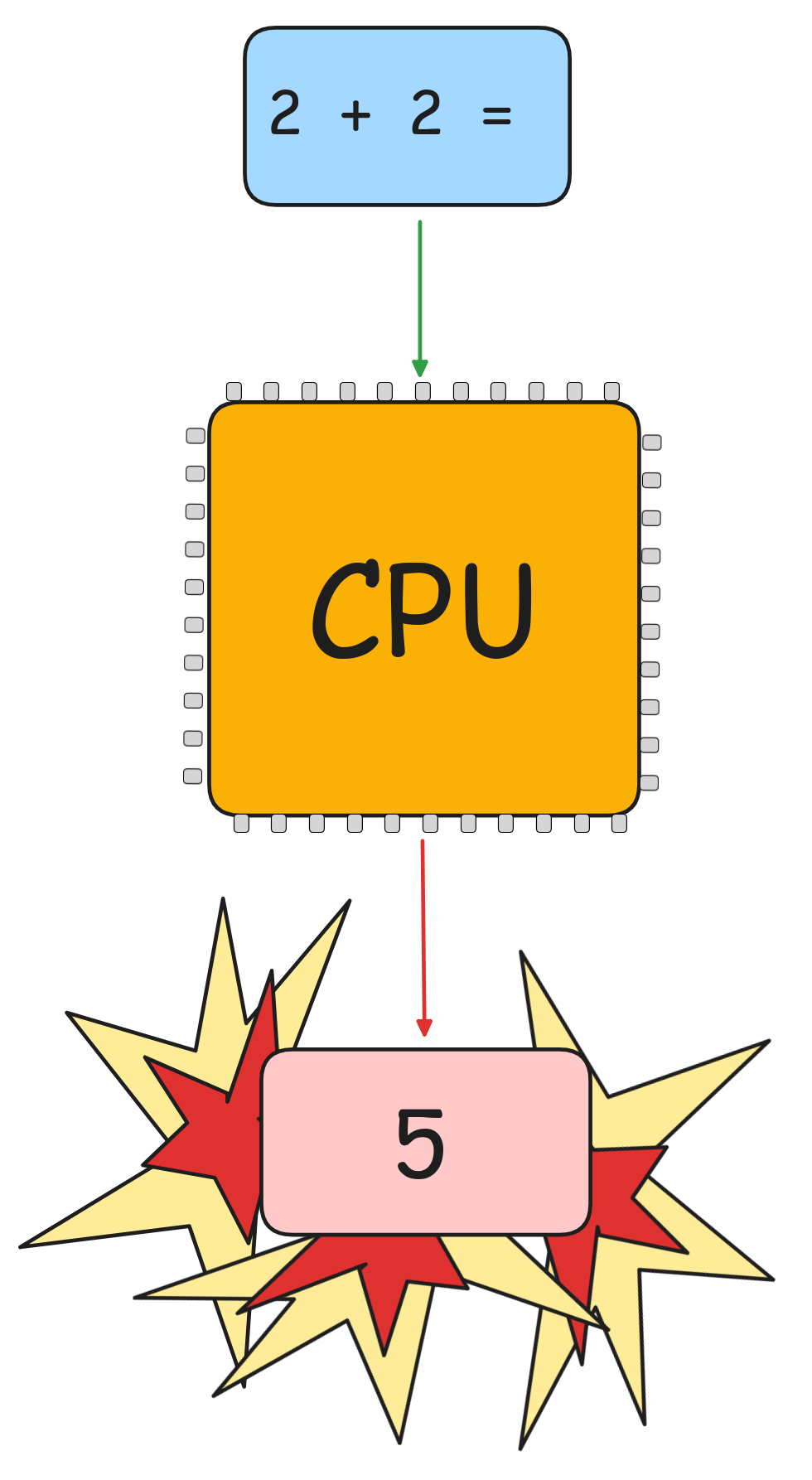
The importance of these technologies is illustrated by the Pentium bug, where an implementation mistake lead to calculation errors in in certain division operations. Not only was this catastrophic for Intel’s bottom line, but imagine what could have happened if the chips had been used in critical infrastructure setups where high-level accuracy is crucial…

From a logical perspective, instead, SAT is the foundation of an important approach to artificial deductive inference. Look again at our inference about the weather from last chapter, again:

According to the Boolean implementation of propositional logic, the validity of this inference boils down to the following fact about valuations:

where:

• [(SUN RAIN)] = { v : v(SUN RAIN) = 1 },
• [ SUN] = { v : v( SUN) = 1 }, and
• [RAIN] = { v : v(RAIN) = 1 }

To verify that the inference is deductively valid, we checked that for each valuation v [(SUN RAIN)] [ SUN], we also have that v [RAIN]. We did this by calculating the propositions [(SUN RAIN)], [ SUN], and [RAIN] and inspecting logical space:

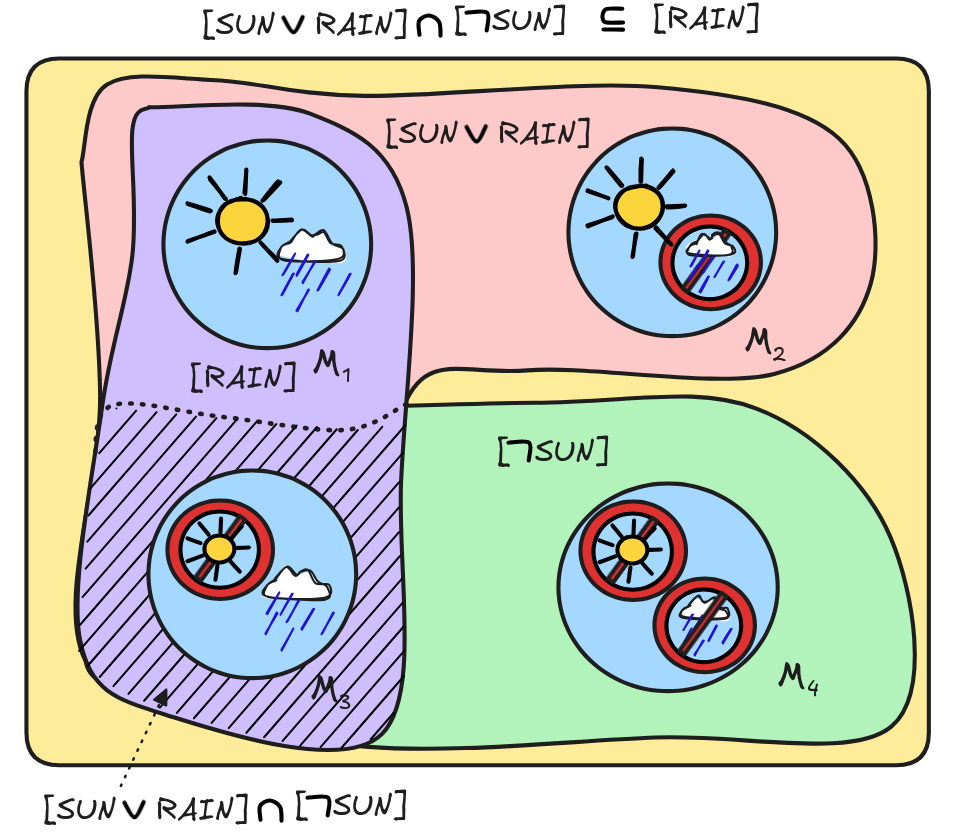
We found that indeed, the only member of
[(SUN RAIN)] [ SUN], viz. the assignment with v(SUN) = 0 and v(RAIN) = 0, is also a member of [RAIN]. This shows to us that every valuation where the premises are true is one where the conclusion is true, i.e.

But we could have asked the question slightly differently and would have gotten the same answer. We could have asked whether there exists a valuation v [(SUN RAIN)] [ SUN] such that v [RAIN]. The answer to this question gives us the same information as the answer to the previous question:

• If there is such a valuation v, it is a countermodel, which makes the premises true but not the conclusion.

• If there isn’t such a valuation v, then every valuation that makes the premises true must make the conclusion true as well.

Just check logical space to help see this: is there any model which is in [(SUN RAIN)] [ SUN] but not in [RAIN]? Of course not! Every element in the former is in the latter.

In the case of an invalid inference, such as our previous example:

this works as well. Working out the relevant propositions gave us the following picture of logical space:

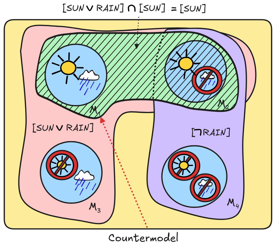
Here we have a valuation v—the one with v(SUN) = 1 and v(RAIN) = 0—such that v makes the premises true—v ([SUN RAIN] [SUN])—but the conclusion is not—v [ RAIN]. The inference is invalid:

Now we just need to make one observation to connect the validity test to SAT, which is that for every formula A, we have that

This mathematical fact derives from the general equation for the values of negations: Combining this with the fact that allows us to see that:

Because no v can be both such that v(A) = 0 and v(A) = 1 at the same time.

So, what we’ve seen now is that to determine whether (SUN RAIN), SUN RAIN is valid, we can ask whether there is a valuation v, such that v [(SUN RAIN)] [ SUN] such that v [RAIN] ("v makes the premises true and the conclusion false"). And by the last observation about the propositions expressed by negations, v [RAIN] means the same as v [ RAIN]. So

is the same as applying the definition of , we can say this even simpler: . So what we’re really asking is whether there’s a v, such that:

If such a v exists, then it is a countermodel to the inference—a model where the premises are true and the conclusion isn’t. The inference is invalid. If no such v exists, the inference is valid, instead.

Now you can hopefully see how the question is related to satisfiability. In logical contexts, we say that a set of propositional formulas is satisfiable just in case there exists a valuation v, which makes all the members of the set true. That is, the validity of

boils down to the satisfiability of

And since this set is unsatisfiable in the logical sense, we can conclude that the inference is valid.

The other inference,

is invalid, instead, since the set

is satisfiable.—In other words, deductive validity and SAT a are two sides of the same coin.

One interesting observation is that the algebraic and the logical interpretation of SAT boil down to, essentially, the same thing. To see this, let’s look at the satisfiability of:

A satisfying valuation v would need to be such that:

But if we apply to this the implementation of the logical operators and in terms of OR and NOT, respectively, we get a Boolean expression, where the only remnants of logic is the use of v applied to the propositional variables SUN and RAIN:

In fact, if we say X = v(SUN) and Y = v(RAIN), the condition becomes:

That that just asks whether the set

is satisfiable in the algebraic sense, which it isn’t, of course. This is, by the way, why we call SUN,RAIN “propositional variables” in propositional logic.

To sum up, what we’ve achieved so far is to reduce two important problems—hardware verification and deductive inference—to SAT problems. Now, in the next step, we’ll look at how we can automate the search for satisfying assignments. We’ll look at SAT solving.

Truth-tables

---

The naive approach to SAT-solving is brute force: to literally go through all possible valuations and check in each case for the satisfaction of the relevant expression(s).

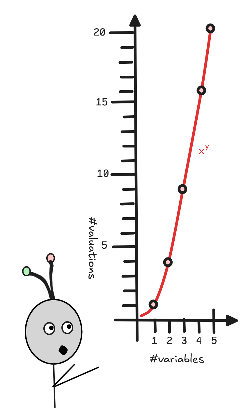Since there can only be finitely many variables (propositional or Boolean) in a given expression, the list of possible valuations is finite: by the rule of products, if there are n-variables, which can take two values each (0 or 1), then there 2ⁿ-many combinations of such values—each being a different valuation. This number grows quickly, in fact exponentially, but it will always be finite. This means that we can go through it. And since a Boolean expression will only ever contain finitely many operations (from NOT, AND, and OR), for each valuation, we only have to carry out finitely many calculations for each formula who’s truth-value we want to know. What this means is that if we have a finite set of Boolean expressions, we can check whether it’s satisfiable in finitely many steps—possibly a large finite number, but finite nevertheless.

A direct consequence of this is that the SAT problem is decidable problem: there exists an effective method, which after finitely many steps generates a correct yes/no-answer to the question whether a given set of Boolean expressions is satisfiable. Since deductive validity in propositional logic can be reduced to a SAT problem, this means that propositional logic is a decidable logic—we can algorithmically automate checking for valid inference in propositional logic.

A procedure for deciding a problem—that is, giving a correct yes/no-answer in finitely many steps—is called a decision procedure. The truth-table method is such a decision procedure, which implements the naive approach described above is an algorithmic fashion.

We can present the method in an algebraic or in a logical fashion. Here we chose the logical flavor, but it will hopefully be clear how to carry out the method in an algebraic fashion.

To describe the method, let’s suppose that we have a set of formulas, of which we want to know whether it is satisfiable. For concreteness sake, we take our running example again and check for the satisfiability of:

The first thing we need to do is to determine all the possible valuations. By what we said above, all we need to do is to count the number of different propositional variables in our set. In our case, #variables = 2. This means that there are 2² = 4 different valuations to consider.

We need to write these valuations down in some order. We typically do this as follows:

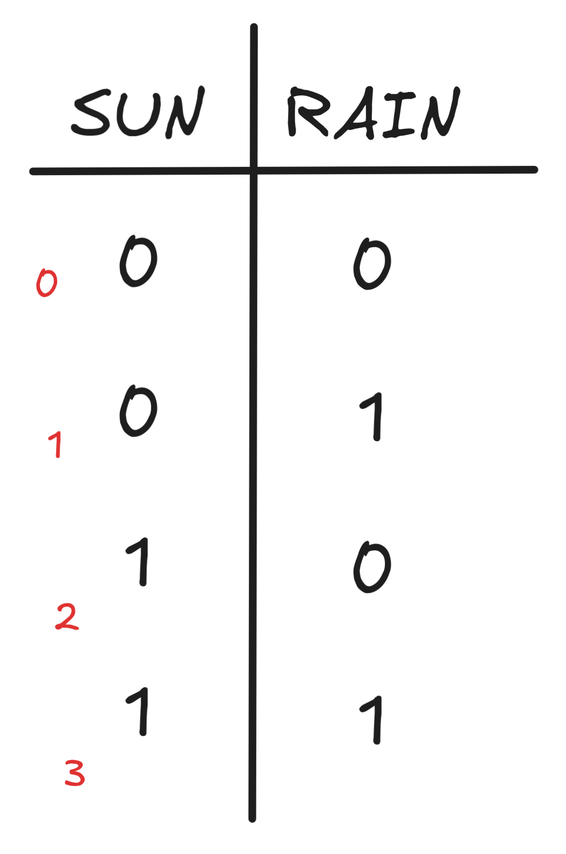
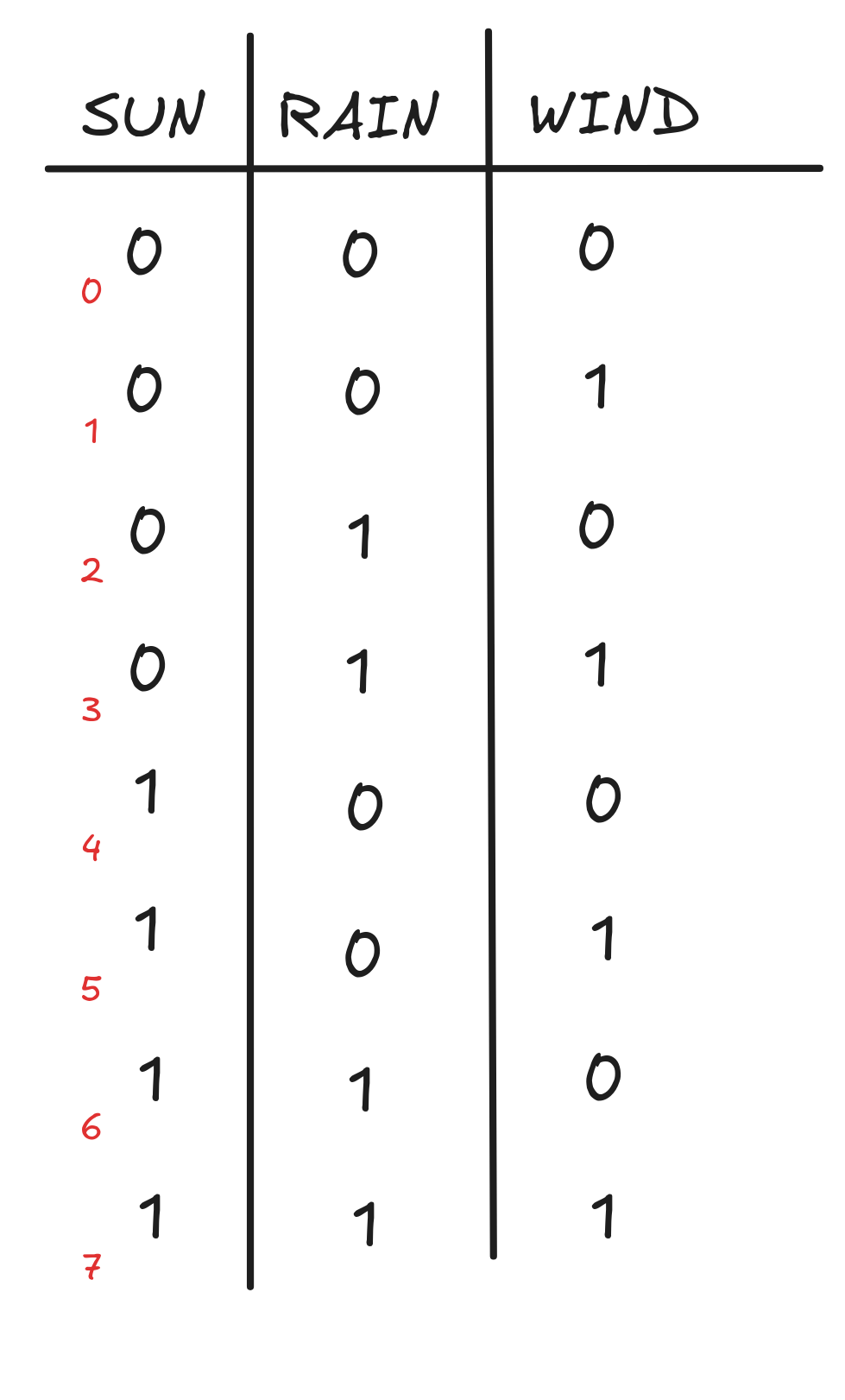
The idea is that each row is a function table for one possible valuation. The red little numbers are not part of the official table, but they illustrate a nice little trick: if you want to determine all the valuations for n propositional variables, just count the rows from 0 to n-1 in binary. In our case, we counted from 0 to 3, which gives us our four rows. But if you have three variables, say SUN, RAIN, WIND, you count from 0 to 7 in binary, and get the following table:

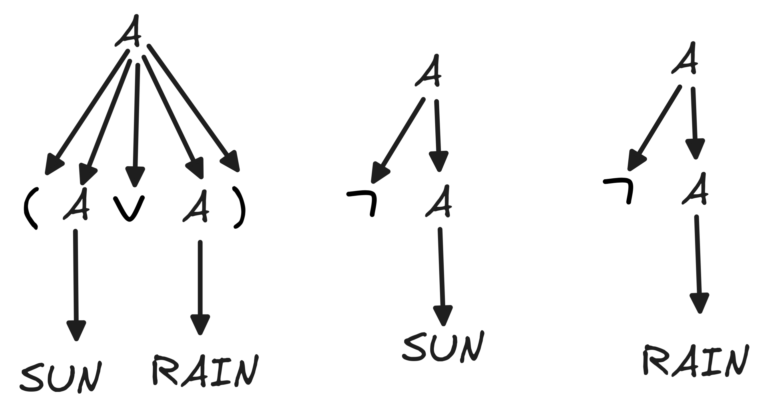
But back to our example with two variables. Next, we need to parse the formulas in our set. This is necessary for an algorithmic calculation of their truth-values. Our case is rather simple. We get:

In the next step, we calculate the truth-values of the formulas under each possible distribution of truth-values. For this, we use the general rules, known as the recursive clauses for the truth-values under a Boolean valuation:

v( A)	=	NOT v(A)
v(A B)	=	v(A) AND v(B)
v(A B)	=	v(A) OR v(B)

We apply these clauses by tracing the parsing tree backwards and calculating the value of the formula generated in the next step by applying the corresponding recursive rule. We don’t worry too much about the concrete implementation of this recursive procedure here, but for this step, the correct parsing of the formula is crucial.

We then document the resulting truth-values in our table like so:

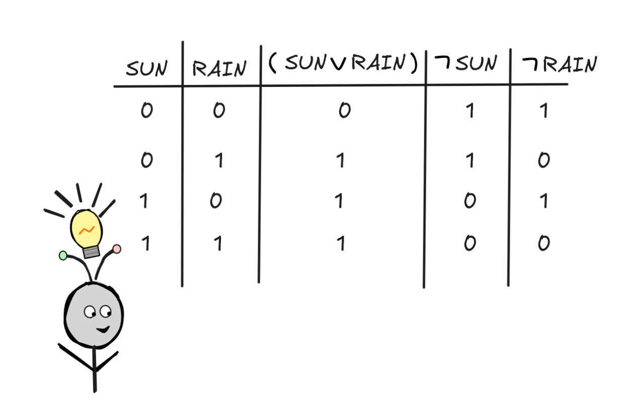
In the last step, we inspect our truth-table and see if we can find a row in which each formula get’s the value 1. If there is one, the set is satisfiable; if there isn’t—like in our case—the set isn’t satisfiable.

This truth-table doubles as the proof of the validity of our inference:

since it shows that the set

is unsatisfiable and the inference thus valid. Note very crucially that the set has an extra where the conclusion occurs—we’re checking whether it’s possible for the premises to be true and the conclusion not true.

For an example of a satisfiable set, let’s take a set with #variables = 3 and some more complex formulas to illustrate a few helpful methods:

The satisfiability of this set corresponds to the invalidity of the inference:

I hope you can see that this is just a more complicated instance of affirming a disjunct*, a fallacy which we’ve mentioned a couple of times before.

The possible valuations, we’ve determined already above. So let’s skip to parsing. The relevant parse trees are as follows:

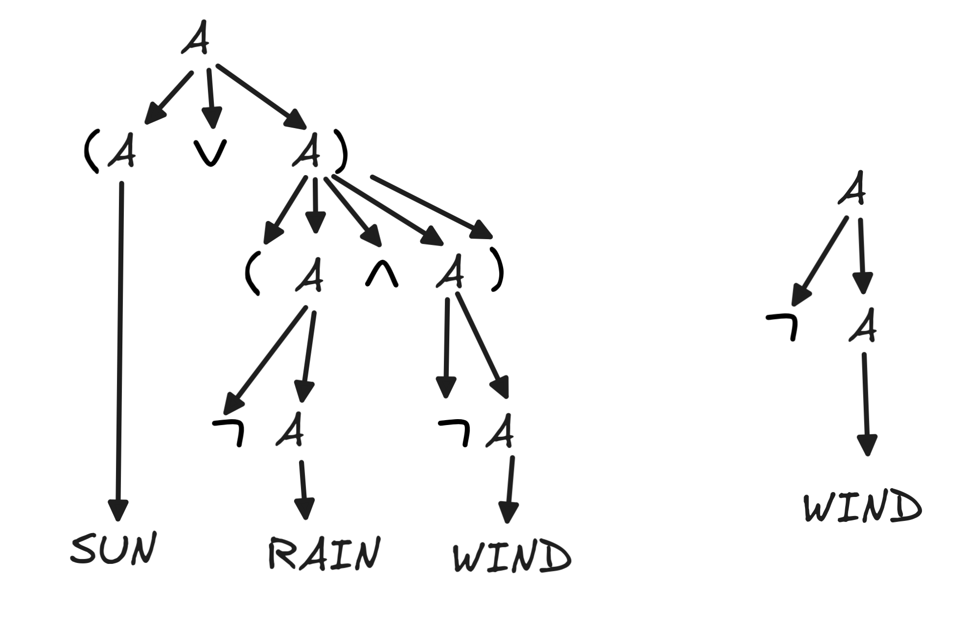
Now in this case, a more complex formula is involved, viz. (SUN ( RAIN WIND)). When we’re calculating it’s value under a given valuation, the parse tree comes in handy. It tells us in which order to apply the Boolean operations NOT, AND, and OR to calculate the truth-values. We can document the calculation in our truth-table as follows:

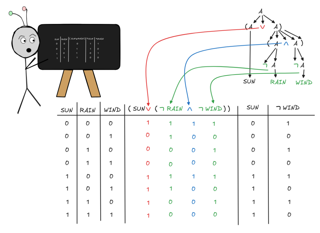
Here, I used color coding and arrows to indicate which recursive step yields which truth-value, but you don’t have to do that every time. You also don’t have to write down the intermediate values, like that of RAIN or ( RAIN WIND), but it can be helpful.

What remains to be done is to check whether there’s a valuation (“row”), where all formulas in the set get value 1. And indeed:

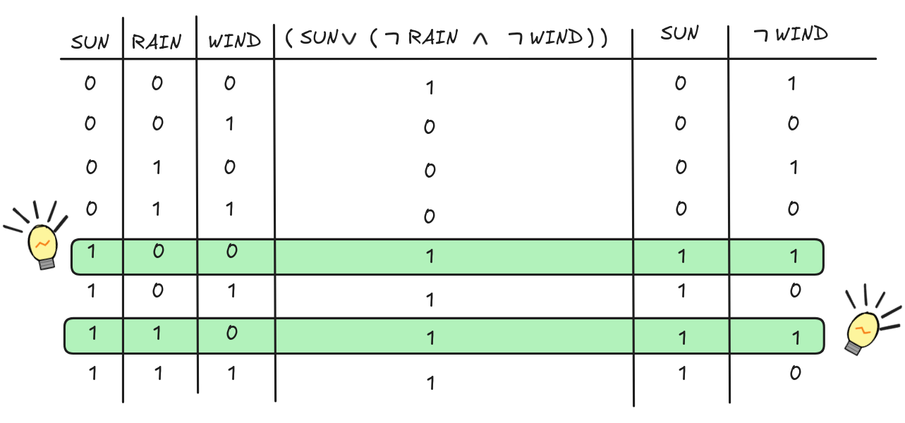
There are indeed two valuations that make all formulas true. But that’s alright, the more the merrier. Either row is enough to show that:

This is, in a nutshell, the method of truth-tables. The method is brute force, but it’s guaranteed to work. The main problem with the method is that how long it takes grows exponentially with the number of inputs. In algorithmic terms, the algorithm has exponential time complexity, which is about as bad as it gets. Using big O notation, the time complexity of the truth-table method is O(2ⁿ), where n is the number of variables involved. Worse even, the way we’ve described the algorithm, we always run for O(2ⁿ)-many steps, since we begin with the computationally most complex step: enumerating the valuations. In this way, truth-tables suffer from what’s called combinatorial explosion.

The aim of other algorithms for SAT-solving is to do better, at least in some cases. It turns out that SAT is connected to very deep problems in computer science and the theory of computation. Finding an algorithm that solves all SAT problems in “significantly less” than exponential run-time would solve one of the most important open problems in theoretical computer science P vs. NP. But the details are out of scope for us.

Normal Forms

---

Many algorithms for SAT-solving make use of so-called normal forms, which are, in a sense, standardized ways of writing formulas or expressions. We can think of it as our “favorite” way of writing a formula in a given context.

The two most important normal forms in logical theory are Disjunctive Normal Forms (DNFs) and Conjunctive Normal Forms (CNFs). Both kinds of normal forms are characterized by a very specific syntactic form. Both Boolean expressions (with variables and operators), as well as logical formulas have normal forms.

We’ve already encountered DNFs when we transformed the truth-table for NAND into a Boolean expression. The result was the expression:

Crucially, this expression was equivalent to the following expression, which we’ve derived from the circuit implementation:

We’ve seen that the two expressions are equivalent in the sense that they always evaluate to the same truth-value for all values for X and Y.

Generally speaking, a Boolean expression in DNF is

• a _disjunction (“chain of OR’s”) of

• conjunctions (“chains of AND’s”) of

• literals (“variables or NOT’s of variables”).

Each chain in this definition can be just have a single element. So, for example:

X, NOT X		NOT NOT X
X AND NOT Y		NOT (X AND Y)
X OR NOT Y		NOT (X OR Y)
NOT X OR ( X AND NOT Y )		X AND ( NOT X OR Y )
(Z AND NOT X) OR ( X AND NOT Y )		X AND ( NOT X OR Y )
⋮		⋮

DNFs are intimately connected with truth-tables. If we have a Boolean expression in DNF, we can “read off” its truth-value distribution from the logical form of the expression:

• Each disjunct, that is each chain of AND’s in the chain of !!OR!’s, corresponds to one way the expression can evaluate to 1.

• To obtain this way, we read an occurrence of a variable as that variable having value 1 and an occurrence of the NOT of a variable as that variable having value 0.

In this way, we can see that

has three ways of evaluating to 1:

• X and Y are both 0, given by the first disjunct ((NOT X) AND (NOT Y)),

• X is 0 and Y is 1, given by the second disjunct ((NOT X) AND Y, or

• X is 1 and Y is 0 given by the third disjunct (X AND (NOT Y)).

In fact, we used this idea “the other way around” to generate the expression: we directly “read it off” off the function table for (X NAND Y).

But the connection between truth-tables and DNFs is very deep. In fact, evidence suggests that working with DNFs doesn’t provide much of an advantage over truth-tables in the context of automated SAT-solving. It turns out that the whether they do once more turns on deep issues like P vs. NP, but from a practical perspective the other kind of normal form, CNFs, have historically been much more fruitful in SAT research.

We’ve described DNFs for Boolean expressions, but we’ll present CNFs for logical formulas. As usual, the notion can be defined for both, but the algorithm we’ll discuss later is more naturally presented in logical terms than directly in Boolean terms.

So, in logical terms, a formula in CNF is a formula which is the:

• conjunction (“chain of ’s”) of

• disjunctions (“chain of ’s”) of

• literals (“variables or their ’s”)

Again, each “chain” in this definition can be just a single formula. So, for example:

RAIN, RAIN		RAIN
RAIN WIND		(RAIN WIND)
RAIN WIND		(RAIN WIND)
RAIN ( RAIN WIND )		RAIN ( RAIN WIND )
(SUN RAIN) ( RAIN WIND )		RAIN ( RAIN WIND )
⋮		⋮

While in a formula in DNF, each disjunct (from “the chain of ORs”) represents one way for the formula to be true, the conjuncts of a CNF are more like a “menu” to pick from. To make a formula in DNF true, one picks one disjunct (that is one literal, a propositional variable or its negation) from each conjunct in the long chain of ’s. Take the following formula, for example:

One way of making it true is to pick SUN from the first conjunct and WIND from the second. That is, the formula is true if the sun shines and it’s not windy. Another way of making it true is to pick RAIN from the first and WIND from the second. That is, the formula is true if it’s neither rainy nor windy. Obviously, we can’t pick RAIN from the first and RAIN from the second. This is not a way to make the formula true, since its not a real possibility in Boolean logic that it both rains and it doesn’t. Excluding these kinds of possibilities from the search space in a systematic fashion is what many SAT-solving algorithms are designed to do.

But before we look at these kinds of algorithms, we need to talk about a fundamental fact about normal forms: there are algorithms for transforming any given expression or formula into an equivalent expression or formula in DNF or CNF respectively. This mathematical fact is known as the DNF/CNF theorem for Boolean logic. In this context, by “equivalent” we mean that for any assignment of values, the original expression/formula always evaluates to the same value as the formula in normal form. Typically, the normal form of an expression is not unique: there is more than one expression in normal form, which is equivalent to a given formula. We can obtain a uniqueness by putting additional constraints, but for now we shall not occupy ourselves with such subtleties.

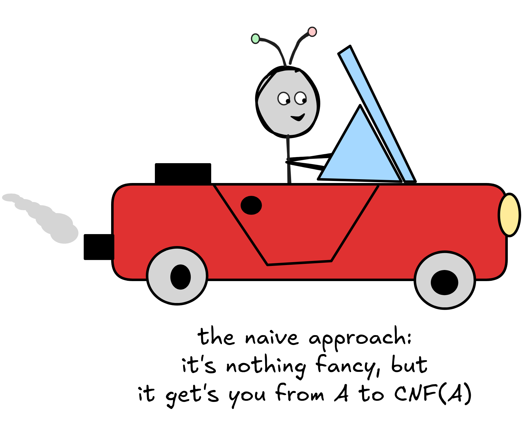There are different algorithms for finding an equivalent formula for a given formula. In practice, we’re interested in transforming a given input as quickly and efficiently as possible, but for now we’ll focus on the naive approach, which though not efficient is straight-forward. When we’re implementing efficient SAT-solvers, we’ll rather use something like the Tseytin transformation, for example, which transforms a formula into a formula that is not necessarily equivalent but at least equi-satisfiable with the original formula: the two formulas can have different truth-values under some assignments, but the original formula is satisfiable if and only if the normal form formula is.

We describe the algorithm for transforming a formula into normal form using rewrite rules, which are similar to the ones we used in our definitions of grammars for formal languages. But rather than rewriting basic expressions into complex formulas, our new rules apply transformations to existing formulas to change them step-by-step from into normal form.

The algorithms for transforming into CNF and DNF both start with the same three rules:

These rules are applied recursively, which means they are not only applied to a full formula, but repeatedly to all subformulas during the entire transformation.

This idea is illustrate in the following re-write sequence:

These rules “push” the negation “inwards”: formulas which begin with a negation are replaced with equivalent formulas where the negation is “closer to” the variables. Note that by the Boolean laws of “Double Negation” and the “De Morgan Identities” the formulas we’re replacing the originals with are indeed equivalent.

Both for converting into DNF and for CNF, we apply these rules until we can’t anymore. The next step is different for the two:

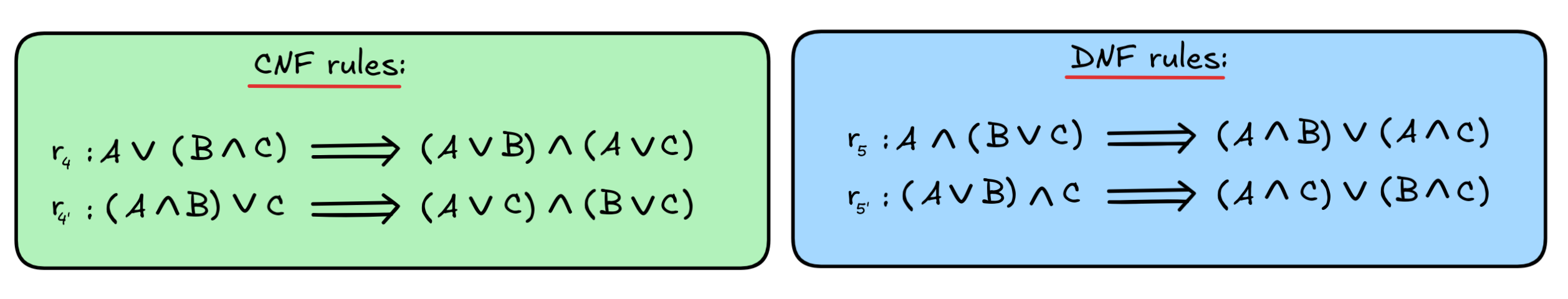
Let’s look at the CNF rule and leave the DNF rule as an exercise. With r₄, we can continue our example as follows:

The resulting formula (SUN RAIN ) (SUN SUN) is in CNF: it’s a conjunction of disjunction of literals.

For what we want to do next, we could stop our transformation at this point. The only thing you might find odd is that we have (SUN SUN) as our second conjunct in this CNF. This is harmless, but we could further simplify using rewrite rules like the following:

With these rules, we continue as follows:

In this way, we can obtain what’s called a canonical normal form, which is unique. Although, there’s one idea missing, which we’ll discuss in the exercises…

We’re now in a place to convert formulas into CNF, which is the starting point of many SAT-solving algorithms. As we mentioned, in industry applications, we’d typically use more efficient algorithms, like Tseytin transformations. But the naive recursive re-write method gets the job done. It’s worth pointing out, however, where the inefficiency lies with this method. Note that in the step where we applied r₄, our formula got longer. In the worst case, this can happen multiple times during a transformation, leading to every growing formulas, where the CNF or DNF is significantly longer than the original, non-canonical formula. This “exponential blowout” is a main roadblock for practical applications.

Resolution

---

One of the main algorithms for SAT-solving in logic-based context is based on resolution, which is a rule of inference that operates on CNFs to determine whether a given set of formulas is satisfiable. We shall now describe how it works.

The starting point for the algorithm is a set of formulas that we want to test for satisfiability, and the 0th step of the algorithm is to transform all of the formulas in the set into CNF. In the following, we assume that this step has been carried out.

For concreteness sake, let’s start with our very simple example of the inference:

We know that this inference is valid just in case the set

is unsatisfiable. As luck will have it, all the formulas in our set are already in CNF, so we don’t have to do anything for the 0th step.

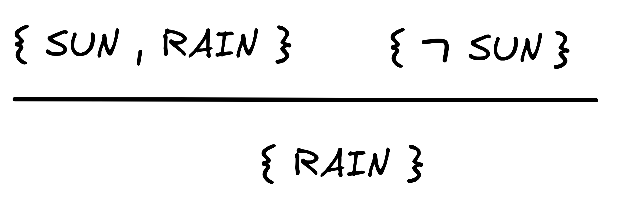
To begin the algorithm, we first transform all the formulas inside the set themselves into sets. It is possible to define the algorithm purely on formulas, but it is easier to work with sets. In our case, the resulting sets are:

The idea is that we turn each conjunct of each formula into a set—the set of its disjuncts and we consider all these sets as the starting points.

If our set would have contained

as well, we’d have to add the following two sets:

The resolution rule is a rule of inference, which allows us to derive new sets from the sets we already have in our collection. For example, the rule allows us to reason as follows:

What is going on here is that we have to complementary literals in the two sets: SUN and SUN. The resolution rule removes this pair and infers the set that contains the remaining literals from both sets.

That is, if our sets had been { SUN, RAIN } and { SUN, WIND }, respectively, the result would have been { RAIN, WIND }.

The idea behind the resolution rule is that to make each formula in our initial set true, we need to make at least one disjunct of each conjunction of each CNF true. In our case, we need to make at least one formula from { SUN, RAIN } and one formula from { SUN } true. But that formula can’t be SUN, nor can it be SUN—because making the one true makes the other false and vice versa. So, we can eliminate the pair SUN, SUN from consideration and leave the others as live candidates, which is what the resolution rule does.

This inference is also called “clausal resolution”. The resolution method consists in repeatedly resolving, while adding the results to our initial set. If we ever get across a set of like

we can kick it out from our search, since it is trivially satisfied and doesn’t constrain our search (keeping it around might get us into loops, but that’s another story). We keep doing this until one of two things happens:

1. We end up with an empty set { } of clauses.

2. We cannot resolve any further.

If the former happens, we infer the initial set is unsatisfiable. This is reasonable because we have arrived at the conclusion that we need to make at least one formula from { } true to make the whole set true, but this is impossible. If, instead, the latter happens, we can pick a member from each set to make true and we infer that the original set is satisfiable. The way in which we do this is something we’ll discuss at another occasion, but for now we leave it at that.

If we continue applying the rule in our case, resolution yields the expected result:

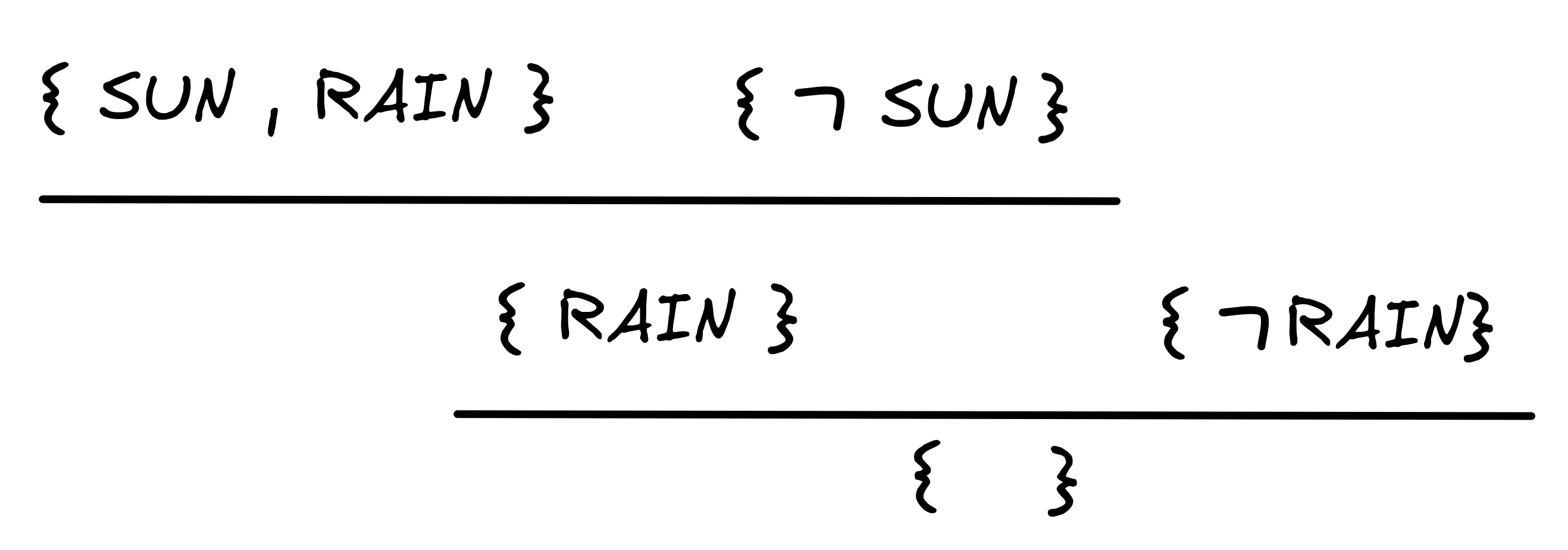
We can derive the empty set { } to witness the unsatisfiability of:

and corresponding validity of the inference in question:

Let’s apply the method to our invalid inference, instead:

To check for validity, we need to check the following set for SAT:

We need to do a simple application of r₁ to transform RAIN into its CNF RAIN, and transforming to sets, we get:

But to this collection of sets no resolutions can be applied.

In fact, if we inspect this list, we can see that there’s precisely one way of picking a member of each set: pick SUN from { SUN, RAIN } and { SUN }, as well as RAIN from {RAIN }. This gives us our final countermodel v with v(SUN) = 1 and v(RAIN) = 1—the same as before, but now we found it in a mechanized fashion.

The resolution method described like this is a sound and complete decision procedure for satisfiability in the sense that for any set of formulas it correctly determines in finitely many steps whether the set is satisfiable. In many cases, it does so much quicker than the truth-table method. For example, in our valid inference, two applications of resolution where enough, even though we needed to check four valuations using truth-tables.

Worst-case the method performs as bad as truth-tables. One bottle-neck is the translation into CNF, which we’ve seen can have exponential blowout. But even if we use smart methods, like Tseytin transformations, resolution might still need many applications of the resolution rule to get the desired result: especially when it comes to satisfiable sets, where we need to go through every case.

In any case, resolution is one of the main methods of SAT-solving, which is the basis for state-of-the art artificial reasoning technologies, like Prover9, Z3, and Vampire. These systems are regularly used for hardware verification and artificial inference. But once we’ve enriched our language with conditionals, we can even use it for activities such as AI planning.