By: Colin Caret and Johannes Korbmacher
Valid inference
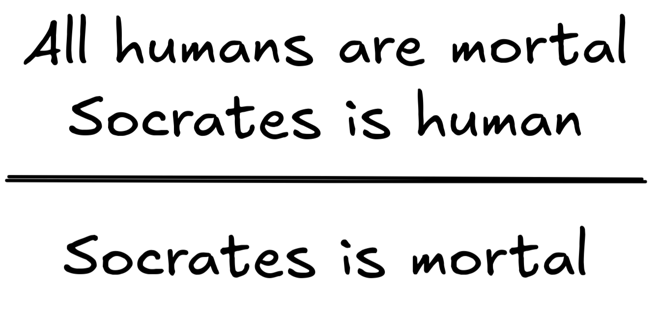
Inference is everywhere in AI. We’ve seen how deductive inference occurs on the level of circuits using Shannon’s interpretation, we’ve mentioned that LLMs use a form of inductive inference to predict pieces of text, and, of course, any artificial general intelligence (AGI) would need to be able perform valid inferences, like our first example:
So what precisely makes an inference valid? What distinguishes good from bad inferences, both in deductive and inductive reasoning?—In this chapter, we’ll deep dive into the logical theory of valid inference.
At the end of the chapter, you’ll be able to:
- explain the relevance of logical form to valid inference,
- explain the difference between material (domain-specific) and logical (domain-general) validity
- distinguish deductively valid from invalid inferences in terms of truth-preservation
- distinguish inductively strong from inductively weak inferences in terms of probability raising
Correctness
When we talk about validity, we are talking about a good feature of inferences, but this is not the only good feature an inference can have. For example, it is good for inferences to be simple, clear, precise, economical, etc. Logic does not deal with all of these topics. Most of these topics are part of rhetoric, the study of persuasive writing style. Logic deals with validity.
Validity is a standard of correctness for inferences. To really fix this concept, it might help to think about it from the other direction. What happens if an inference lacks validity, when it is invalid? Well, that shows us that something went wrong. The inference made a mistake. Some of these logical mistakes or fallacies are so famous that they have their own names.
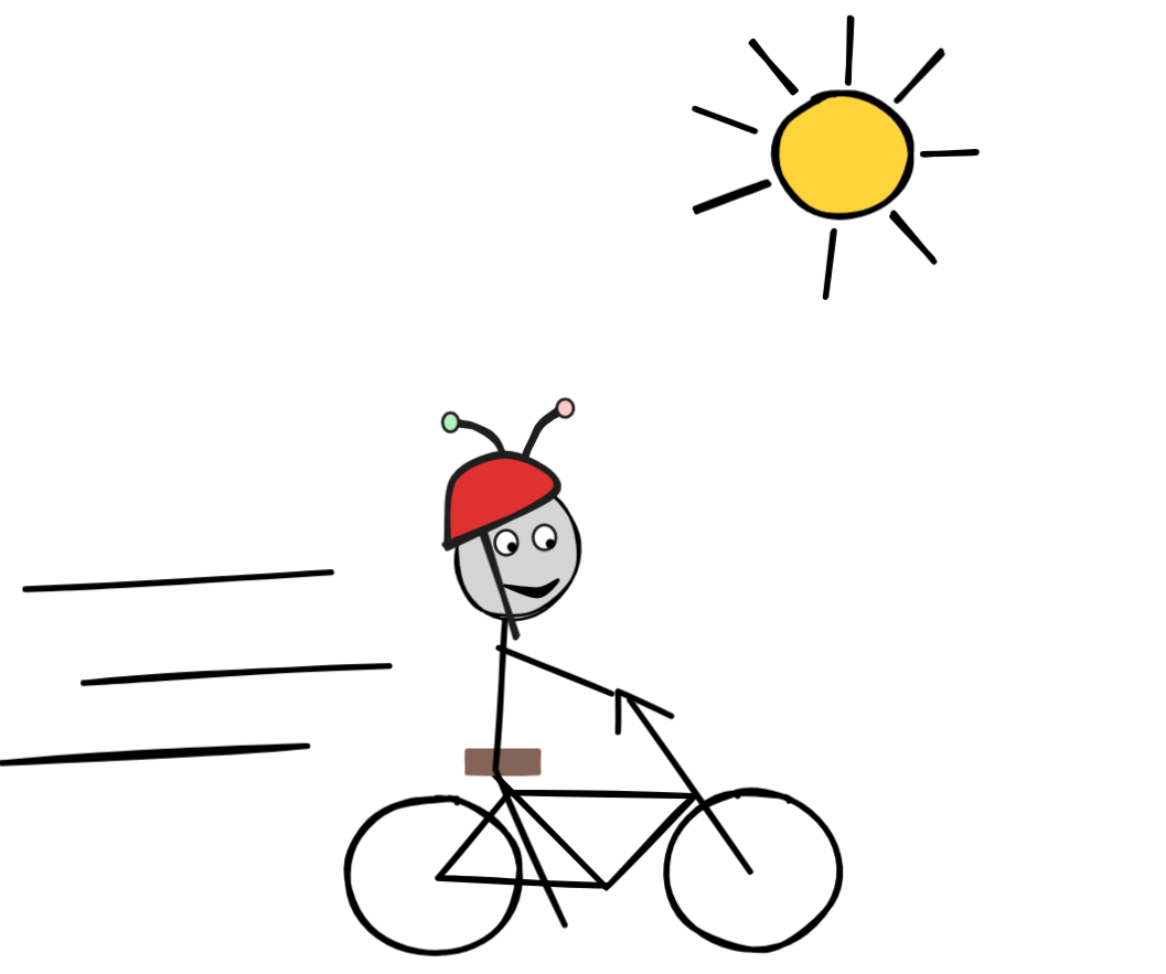
Here is an example of a fallacy called affirming the consequent:
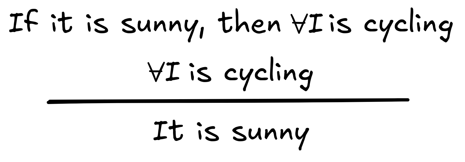
 The mistake should be clear. The
conditional premise says that sun leads
to sport. However, the other premise of this inference is not about sunny
weather, so those two premises don’t really “add up” to anything useful. They
certainly do not support the conclusion that it is sunny today.
The mistake should be clear. The
conditional premise says that sun leads
to sport. However, the other premise of this inference is not about sunny
weather, so those two premises don’t really “add up” to anything useful. They
certainly do not support the conclusion that it is sunny today.
Contrast this with the following valid inference:
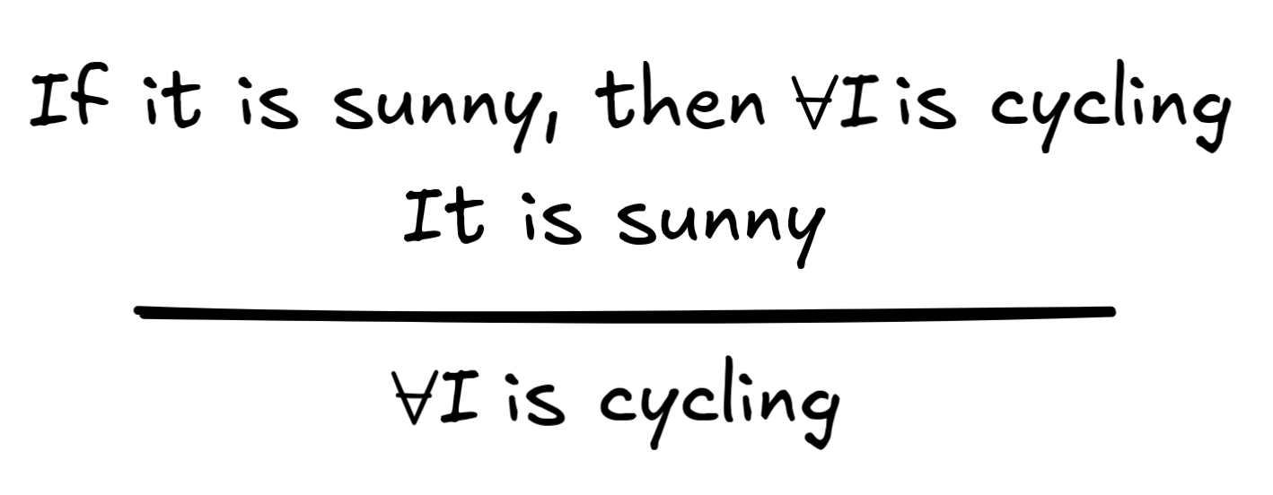
This inference involves a premise about sunny weather, which connects with the
conditional premise in the right way. This inference is valid because it uses
all of its premises correctly. These two examples show that it can be easy to
confuse valid and invalid inferences if we don’t pay attention to the details.
At a glance, the two inferences look pretty similar.
This is why logic aims for a systematic definition of validity. This notion should be applicable not only to humans but to any information-processing system. It can tell us what counts as intelligent behavior. Without a definition of correct reasoning, how do we even know what we want AI to achieve?
So, we would like to say, in general, what makes an inference valid or invalid. The standard idea is that valid inferences preserve truth from their premises to their conclusion.
Hypothetically
To test whether an inference is valid, we ask if the conclusion is true when the premises are true. This is a hypothetical question. Answering this question does not require us to know that the premises really are true. In fact, we can make a stronger point: it is possible to have an inference that is valid even though it has false premises. Here is an example.
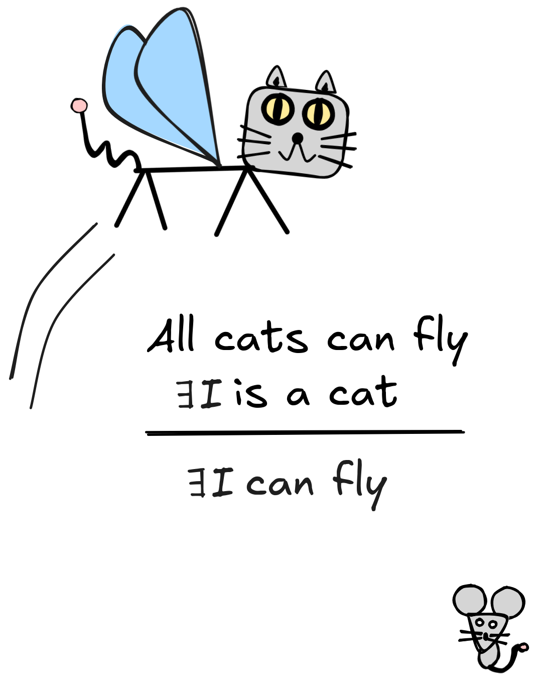
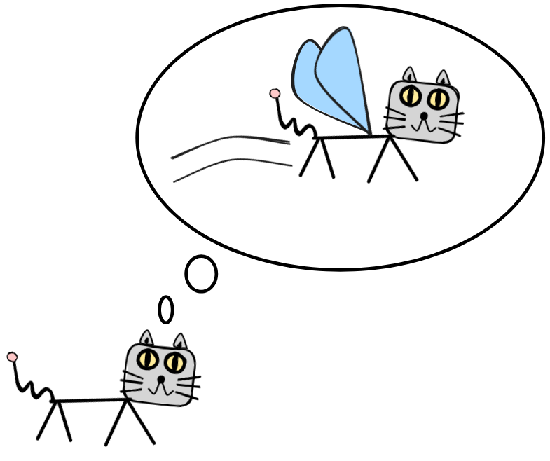
The reasoning behind this inference is perfectly correct. The conclusion follows from the premises. That makes the inference valid. But we obviously know that this inference also involves some false premises. Cats can’t really fly.
The important point is that validity is not determined by the actual truth or falsity of statements. What we care about is the connections between statements.
When we test for validity, we do not look at the actual truth of premises and conclusion, instead we look for a relationship between their truth-values. You can think about it like this: imagine that the premises and true and think about whether the conclusion is true under this assumption.
Think about the inference this way. When we do this, we imagine a world that is slightly different from the actual world, a world where cats do fly. In that kind of world, it has to be true that IE flies.
This is the basic idea of truth-preservation:
An inference is valid iff the conclusion is true under the (hypothetical) assumption that the premises are true.
Now, we can ask a series of follow-up questions. How tight is the truth-preservation relationship? How often does it have to hold? How reliable does an inference need to be in order to call it “valid”? Different answers to these questions take us in two directions: deductive and inductive logic.
Formally – Logical validity
Take our first example again:
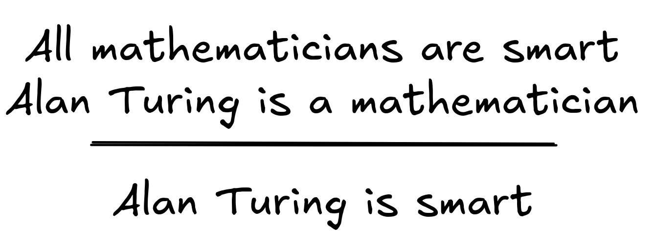
This is, of course, a valid inference: under the assumption that the premises are true, so is the conclusion. But note that for this, it doesn’t matter that we’re talking about Socrates or mortality. If we change the term Socrates to, say, Alan Turing , and we change the predicates human and mortal to, say, mathematician and smart , we’d get the following inference, which is also valid:
Also our example from above about IE
being able to fly is the
result of changing
Socrates
to
 ,
human
to
cat
, and
mortal
to
can fly
. In fact, for every way of replacing terms and predicates like this, the inference remains valid.
,
human
to
cat
, and
mortal
to
can fly
. In fact, for every way of replacing terms and predicates like this, the inference remains valid.
In logical theory, we say that the argument is valid in virtue of its logical
form. We can express the shared logical form of the inferences in question
as follows:
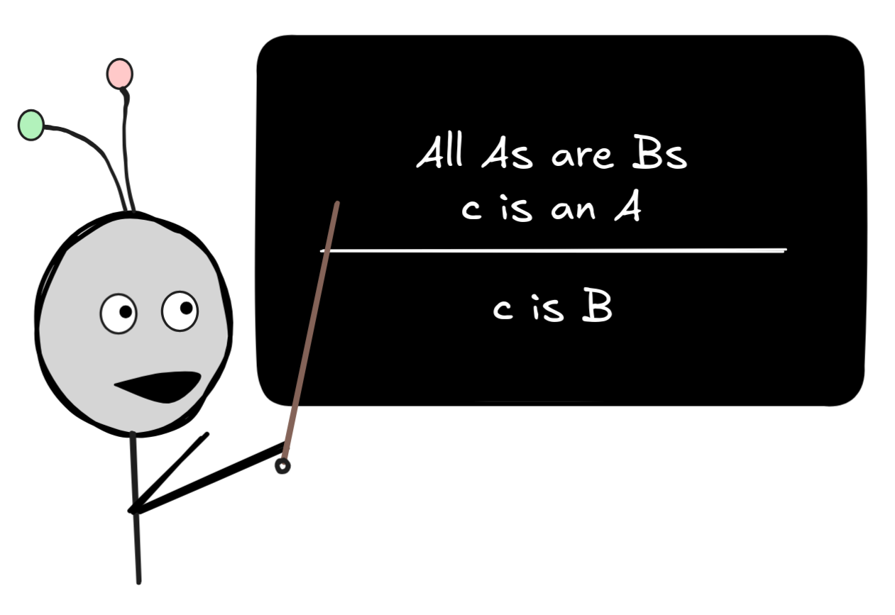 Here, the A and
B are placeholders for arbitrary predicates,
and the lower-case c is an arbitrary term. The
idea is that whichever expressions we put in for
A,B and c, as
long as they’re of the right grammatical category, we’ll get a valid inference.
By representing the logical form of our inference in this way, we’re
abstracting away from the logically irrelevant predicates and terms and obtain
an abstract representation of the logical form.
Here, the A and
B are placeholders for arbitrary predicates,
and the lower-case c is an arbitrary term. The
idea is that whichever expressions we put in for
A,B and c, as
long as they’re of the right grammatical category, we’ll get a valid inference.
By representing the logical form of our inference in this way, we’re
abstracting away from the logically irrelevant predicates and terms and obtain
an abstract representation of the logical form.
So far, we’ve discussed the idea of logical form in natural language. But as
we’ve discussed in the previous chapter, for the purposes of AI research, we
need to work in formal languages. We haven’t encountered a formal language
yet that is expressive enough to represent our inference about Socrates, but we
can illustrate the point with relation to MP, which is the following inference schema, introduced in the previous
chapter:
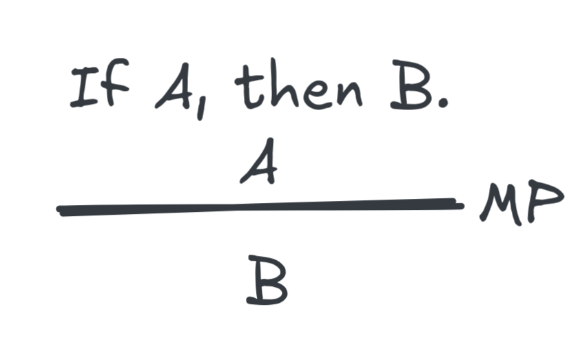 In the language of propositional logic, we can express this logical form more
precisely using the logical operators we’ve introduced in the previous chapter.
Remember that
In the language of propositional logic, we can express this logical form more
precisely using the logical operators we’ve introduced in the previous chapter.
Remember that
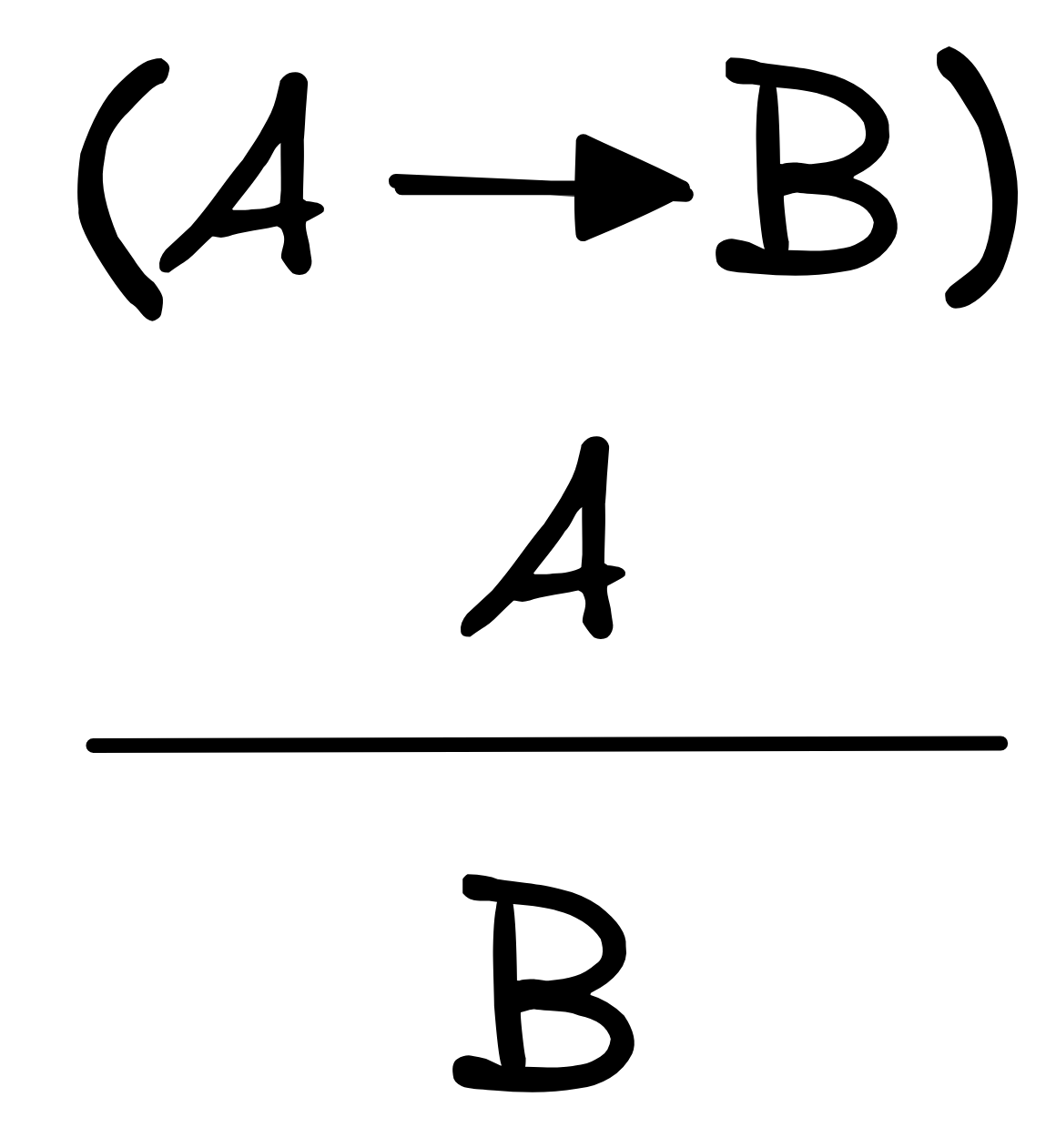
 represents the natural language “if …, then …”. In formal
languages, we let letters like A,B represent
arbitrary formulas, like in the schema we wrote before. So, in purely formal
terms, we can write the inference as:
represents the natural language “if …, then …”. In formal
languages, we let letters like A,B represent
arbitrary formulas, like in the schema we wrote before. So, in purely formal
terms, we can write the inference as:
 To be able to write this in one line, we also use the symbol
 (read “therefore”) in place of the inference line like so:
A, (A
(read “therefore”) in place of the inference line like so:
A, (A
 B)
C
.
B)
C
.
To express the logical claim that MP
is valid we use the logical symbol ⊨, which is
called the “double turnstile” or “models” (for reasons we’ll get into later).
So, we write the validity of MP in purely formal notation as
A, (A
B) ⊨ B
.
By the way, it’s important to distinguish between the inference
A, (A
B)
B
and its validity
A, (A
B) ⊨ B
: there are logical systems where
MP is not valid. In those contexts, an AI system might
still—fallaciously—reason according to MP, i.e. it might apply
A, (A
B)
C
even though, in this context,
A, (A
B) ⊭ B
.
Validity in virtue of logical form, as just discussed, is known as logical consequence. But, importantly, not all valid inferences are logically valid—valid in virtue of their logical form. Consider the following inference, for example:
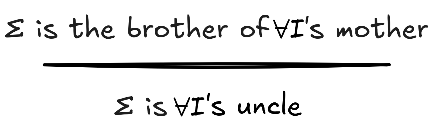
Following the truth-preservation criterion, this inference is certainly valid.
Under the assumption that
 it’s true that
 since an uncle is, by definition, a parent’s male sibling.
But if we replace brother with sister, for example, we get the following invalid inference:
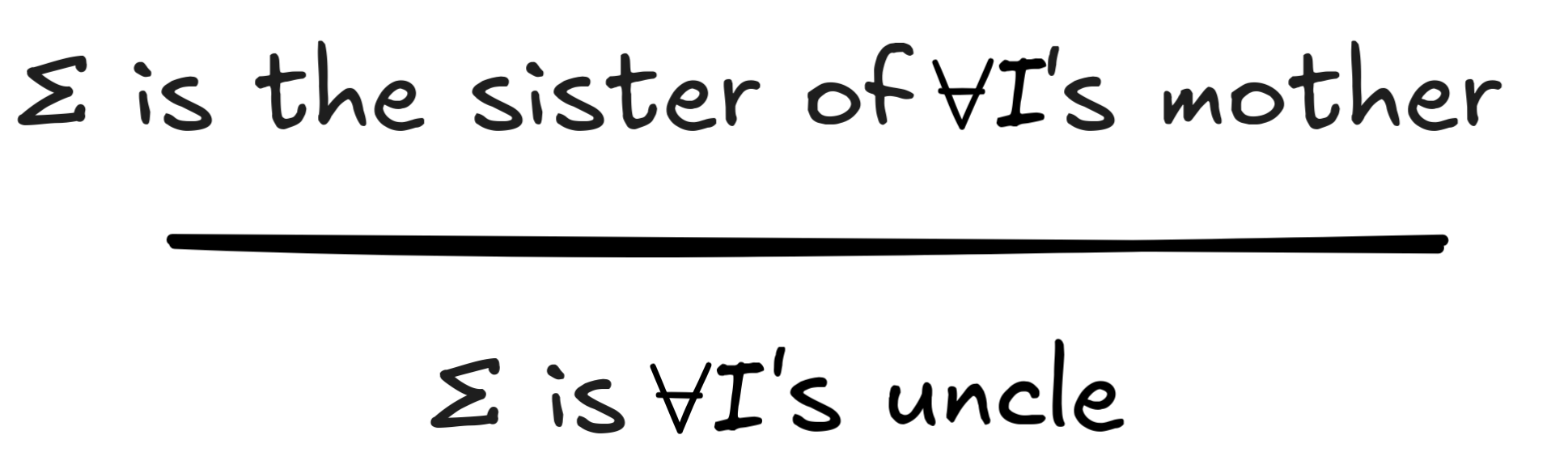 If we assume that Σ is IA
’s mother’s
sister, Σ is IA
’s aunt and not their
uncle. This shows that the inference is not valid in virtue of its form, which
is something like:
If we assume that Σ is IA
’s mother’s
sister, Σ is IA
’s aunt and not their
uncle. This shows that the inference is not valid in virtue of its form, which
is something like:
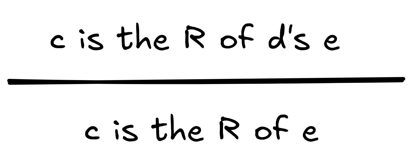
But the inference is valid … in a sense. The validity of the inference depends on the concrete predicates involved—the meanings of brother, mother, and uncle. In logical theory, we also call inferences like this, which are valid, but not in virtue of their logical form, materially valid. While logical validity—validity in virtue of logical form—is is domain-general, material validity is domain-specific. As we’ve seen, for the validity of our inference about Socrates it doesn’t matter that we’re talking about Socrates, being human, or being mortal, but for the validity of our inference about IA ’s uncle, it does matter that we’re talking about his mother’s brother and not sister.
This means that the classification of valid inferences we’ve discussed before needs to be further qualified on the deductive side:
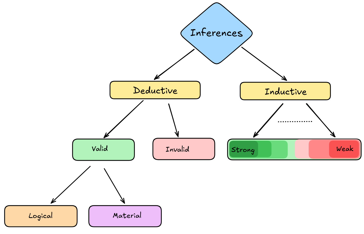
The distinction between domain-general and domain-specific inference is crucial to understand some recent advances in AI research: while LLMs are getting better and better at domain-specific inference, such as inference in mathematics, they are still underperforming in domain-general, logical inference. Some researchers speculate that improving the domain-general reasoning abilities of AI systems improves their domain-specific reasoning abilities as well.
There is close connection between logical and material validity. Some
logician’s, like
Rudolf Carnap,
have suggested that we can reduce material validity to a special case of
logical validity under additional assumptions, so-called “meaning postulates”.
His idea is based on the observation that the material validity of the inference
about IA
’s uncle can be expressed in the logical validity of the
following inference:
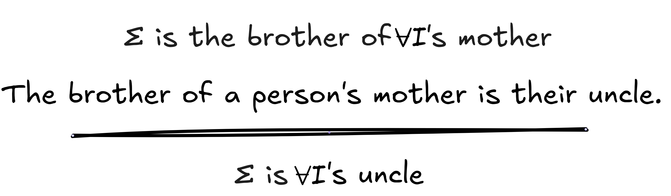 Here the statement
the brother of a person's mother is their
uncle
is a meaning postulate, which captures (part of) the
meaning of the term
uncle
.
While
Here the statement
the brother of a person's mother is their
uncle
is a meaning postulate, which captures (part of) the
meaning of the term
uncle
.
While
Always – Deductive validity
We’ve previously defined a deductively valid inference to be one where the premises necessitate the conclusion. We can think of this as stipulating that truth-preservation always holds. In deductive inferences, we want 100% reliability in all situations whatsoever. No exceptions allowed. Necessarily, in any situation where the premises are true, the conclusion is true as well. Otherwise, if there’s a situation where the premises are true and the conclusion isn’t, the inference is deductively invalid. This is a high standard we are asking for but it is very useful when we can identify this kind of air-tight reasoning.
 Deductive reasoning is characteristic of mathematical inference, which we
encounter not only in pure math, but also in applications of mathematics in
physics and the natural sciences. When we make predictions, for example, about
the trajectory of an asteroid heading towards earth, this involves a lot of
deductive, mathematical reasoning. We start with some empirical observations
and apply physical laws, but the actual calculation is deductive. That means
that, assuming the calculations are carried out correctly, the result is as
certain as the observation: the only reason why the prediction could be wrong
is that the assumptions—the laws or observations—are wrong.
Deductive reasoning is characteristic of mathematical inference, which we
encounter not only in pure math, but also in applications of mathematics in
physics and the natural sciences. When we make predictions, for example, about
the trajectory of an asteroid heading towards earth, this involves a lot of
deductive, mathematical reasoning. We start with some empirical observations
and apply physical laws, but the actual calculation is deductive. That means
that, assuming the calculations are carried out correctly, the result is as
certain as the observation: the only reason why the prediction could be wrong
is that the assumptions—the laws or observations—are wrong.
Since the rules for deductive logic are indefeasible, they are suited to belief accumulation. These rules do not vary between contexts. They do not require special justification. There is nothing that can make these rules fail. Nothing can defeat a deductively valid inference.
 The optimal way of using deduction is to take a set of existing beliefs (or
knowledge) and then add more beliefs (or knowledge) by applying logical rules.
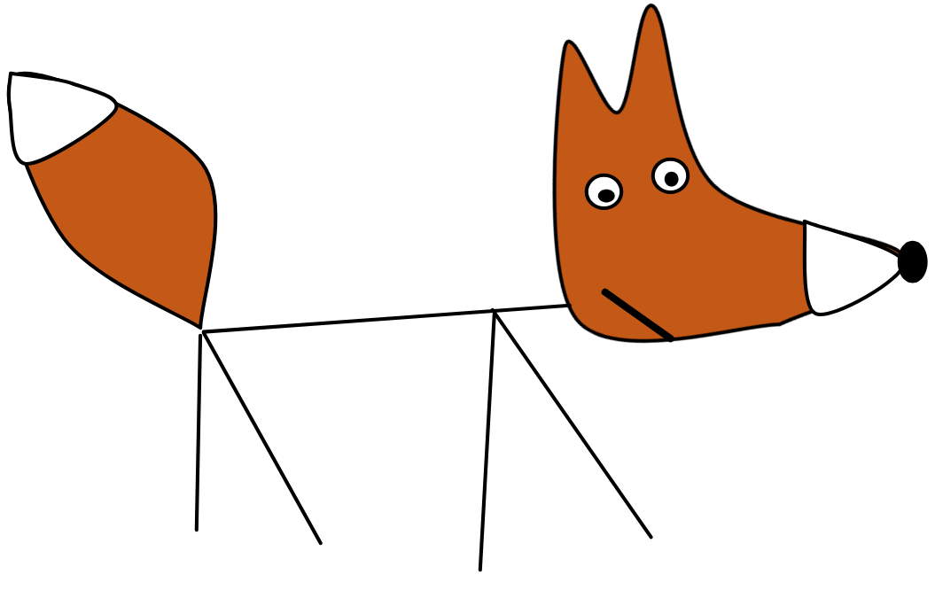
A common, real world implementation of deductive reasoning occurs whenever we
apply some general pattern to a specific case. For example,
vixens are female foxes. That is the
definition of the concept vixen. Suppose you know this and you hear someone
say “there is a vixen living in the forest!”. In that case, you might use
deduction to infer that there is a fox living the forest.—This kind of
deductive inference should be carried out by any reasoning AI system, such as
expert systems, but also reasoning LLMs, such as OpenAI’s
o4-mini or Deepseek’s
R1.
The optimal way of using deduction is to take a set of existing beliefs (or
knowledge) and then add more beliefs (or knowledge) by applying logical rules.
A common, real world implementation of deductive reasoning occurs whenever we
apply some general pattern to a specific case. For example,
vixens are female foxes. That is the
definition of the concept vixen. Suppose you know this and you hear someone
say “there is a vixen living in the forest!”. In that case, you might use
deduction to infer that there is a fox living the forest.—This kind of
deductive inference should be carried out by any reasoning AI system, such as
expert systems, but also reasoning LLMs, such as OpenAI’s
o4-mini or Deepseek’s
R1.
Moreover, many programming languages are essentially formal languages with deductive rules. This is a perfect way to apply logical methods. Consider the code snippet below. This simple Python snipped is supposed to take an input that is a whole number and identify whether it is a positive number or not:
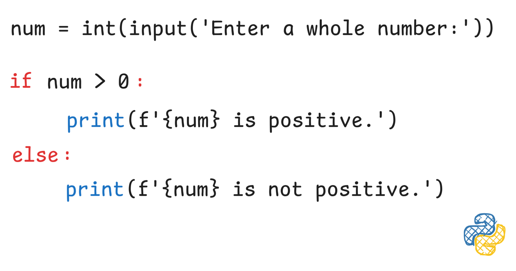
Imagine what would happen if the computer did, effectively, not obey deductive rules like “modus ponens”. We would have no idea what to expect when we run this program. Sometimes when you ran the program and entered the number 1, you might get the correct answer that 1 is a positive number, but other times you might you get no answer at all. That would be useless and frustrating. In order to make the behavior of programs predictable, we want them to effectively follow deductive rules of reasoning.
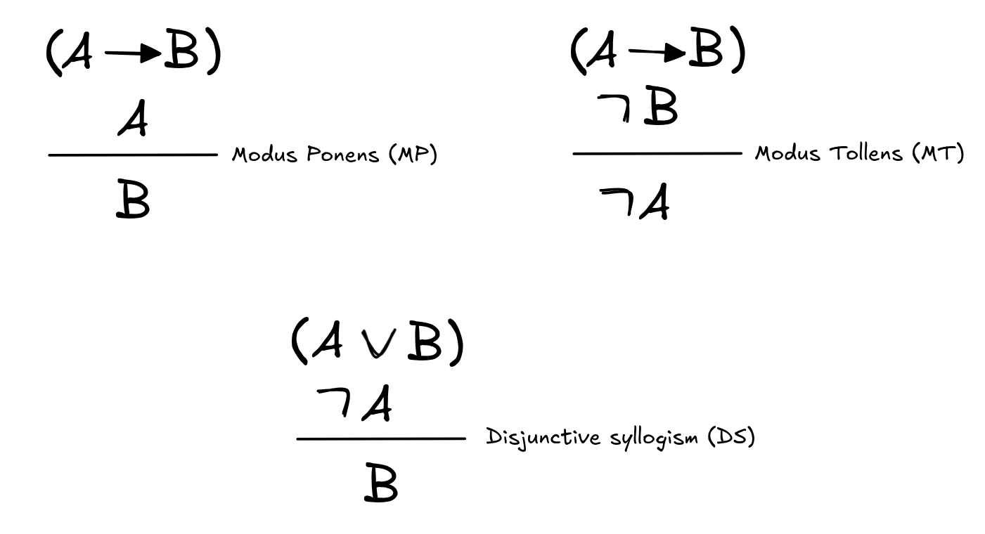
We’ve already encountered some examples of deductively valid inferences, like the one concerning Socrates’ mortality. Here are some further examples of inference schemas, which are often considered to be deductively valid in propositional logic:
Similarly, we’ve seen some inference patterns that may seem deductively valid, but are generally agreed to be fallacies:
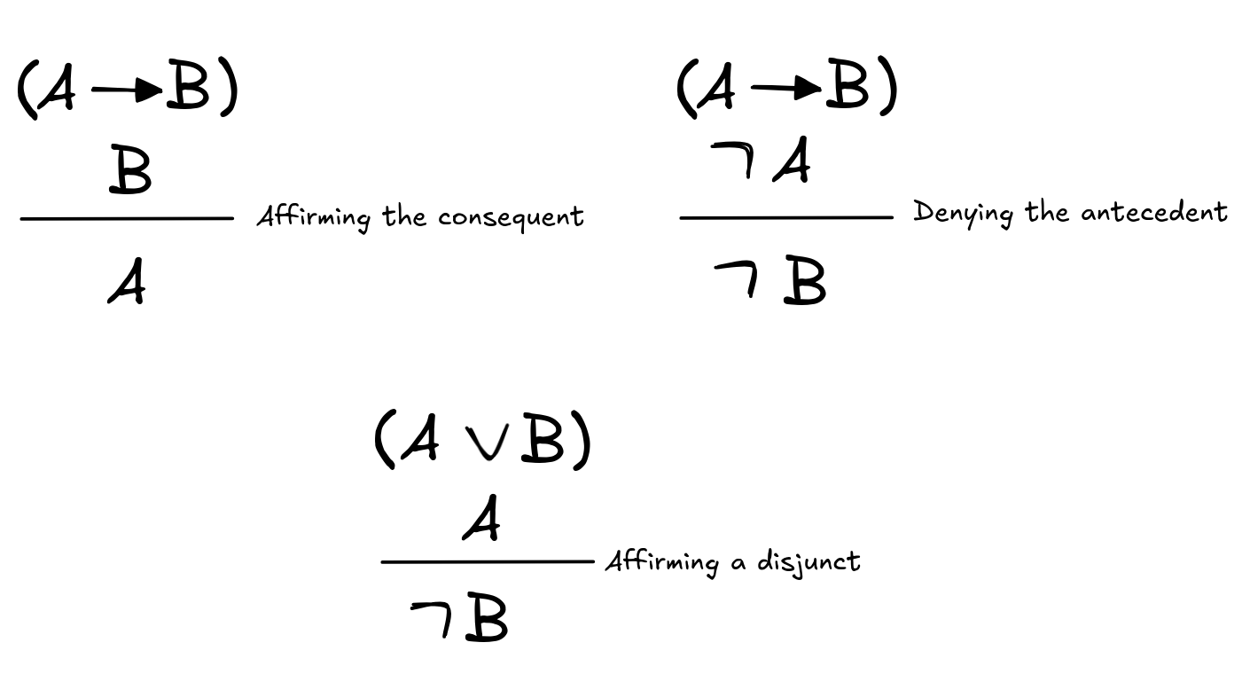
One of the central aims of deductive logic is to provide a theory of deductively valid inference which can account for the apparent deductive validity and invalidity of the above inference schemas.
 The standard approach to developing such an account is the semantic
approach. The basic tool it uses is that of a semantic model. A semantic
model is like a picture of a possible reasoning scenario. Think for example of
the scenario we considered above, where all cats—and thus IE
—could fly. If we look
at a model, we can ask whether a specific sentence
A is true or not in that model. Every model
gives an answer. It assigns a definite truth-value to each sentence. If we take
the sentence
can fly
and consider the scenario, where cats can fly, we get the answer that the
sentence is true. But if we evaluate the sentence relative to the way things
actually are, the answer is that it’s not true.
The standard approach to developing such an account is the semantic
approach. The basic tool it uses is that of a semantic model. A semantic
model is like a picture of a possible reasoning scenario. Think for example of
the scenario we considered above, where all cats—and thus IE
—could fly. If we look
at a model, we can ask whether a specific sentence
A is true or not in that model. Every model
gives an answer. It assigns a definite truth-value to each sentence. If we take
the sentence
can fly
and consider the scenario, where cats can fly, we get the answer that the
sentence is true. But if we evaluate the sentence relative to the way things
actually are, the answer is that it’s not true.
In logical theory, semantic models are defined relative to a formal language and the concrete definition of a model depends on the specifics of the language under consideration. In fact, as we’ll see a lot of work goes into defining the notion of a model with mathematical precision. So, we’ll have to postpone this to later lessons. But what we can talk about is the general pattern that all semantic definitions of deductively valid inference follow.
For this, let’s assume that we’re dealing with a formal language L , defined in terms of an alphabet and grammar, for which we’ve defined the notion of a model, such that for every model M for L each formula A of L is either true or not. Generally speaking, a formal language has more than one model. Different models assign different values to the same sentences. In one model perhaps A is true and B is not. In another model B is true and A is not. That variation allows models to picture different scenarios.
Now it’ll be helpful to talk about sets again. Remember that a set is collection of arbitrary objects, anything can be in a set—even abstract mathematical objects like models. So for each formula A , we can consider the set of models where the formula is true. We write this as [A] . Using the set-theoretic notation we introduced when talking about formal languages, we can write an explicit definition of this set using set abstraction:
[A] = { M : M is a model, where A is true}
It can be helpful to imagine this set as part of a logical space of models. In the diagram below, we assume that every model M for our language L “lives” in the yellow rectangle. We depict them as little blue balls or “worlds”. The green set (region) inside it is the set of all models where A is true, i.e. [A] :
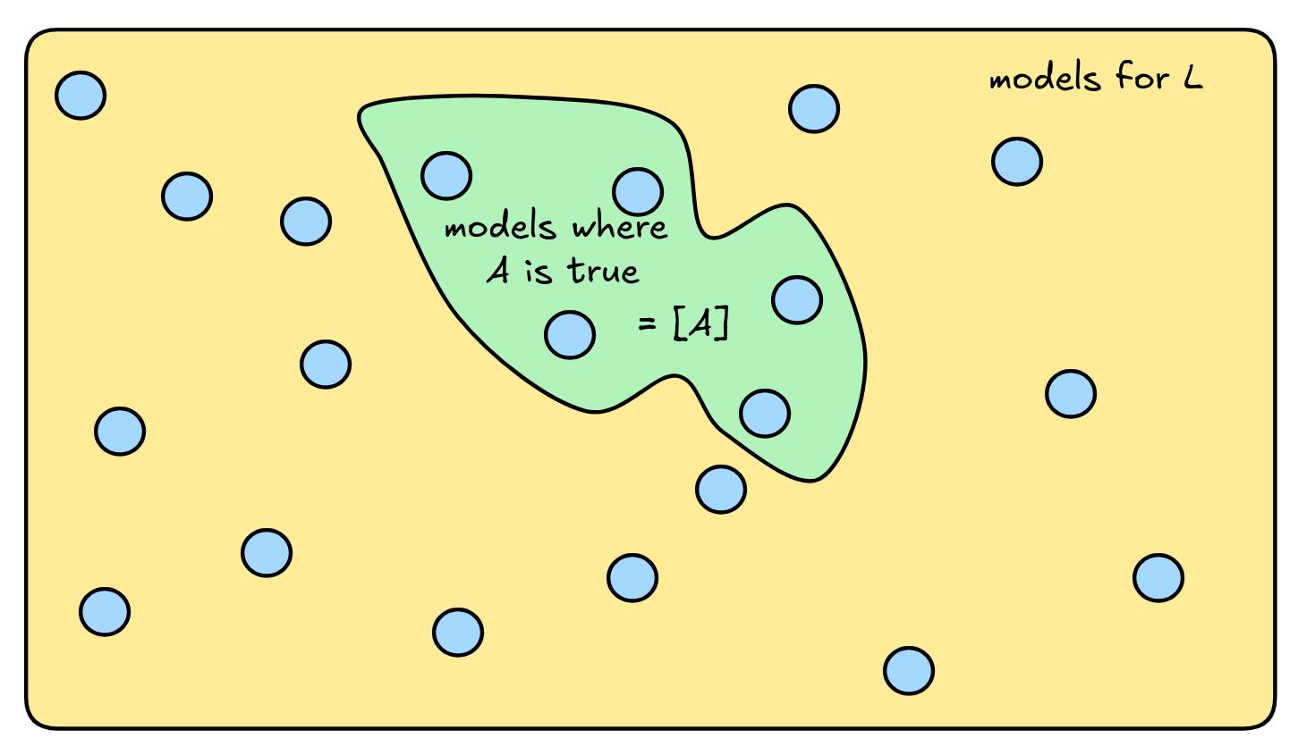
The set [A] is also called the proposition expressed by the formula A . The set [A] represents, as it were, the semantic content of the formula A from a logical perspective.
We can use this picture of logical space to define the notion of deductively
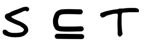
valid inference, but first we need another bit of set theory. When all the
members of one set,
S
, are
also members of another set,
T
, we say
that the set
S
is a subset of
T
. Symbolically, we write:
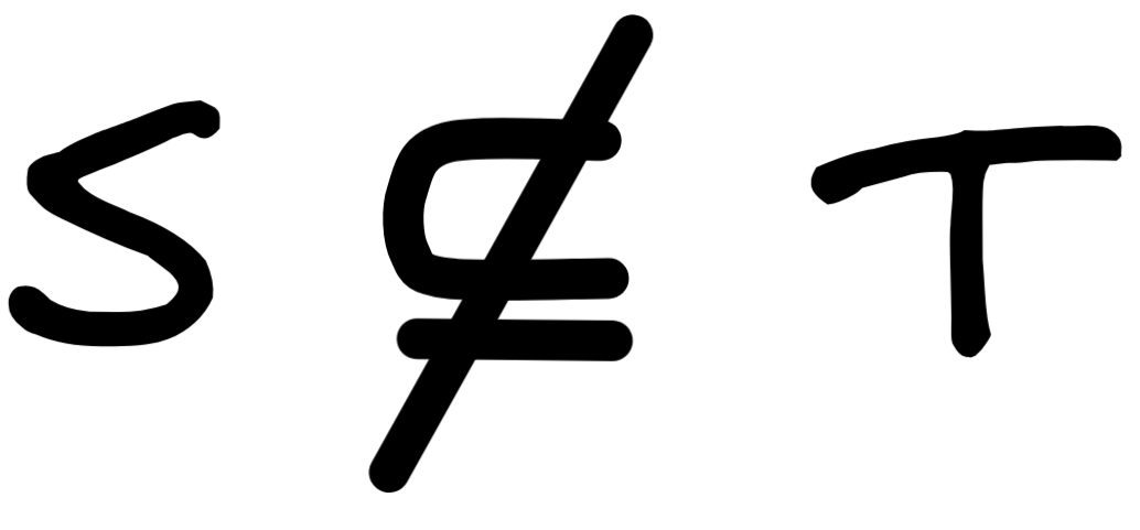
 . When there is at least one member in
S
that is not in
T
, then
S
is not a subset of
T
, symbolically:
. When there is at least one member in
S
that is not in
T
, then
S
is not a subset of
T
, symbolically:
 .
.
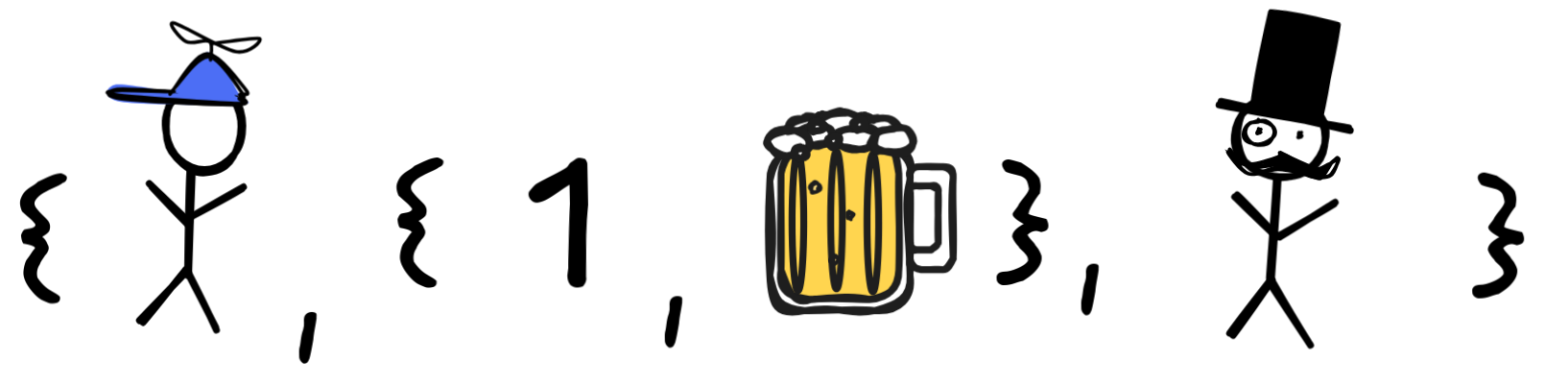
Take, for example, the set that contains little Jimmy, the set that contains the number one and my beer, as well as Mr. Sir:
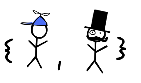
Then consider the set that contains only little Jimmy and Mr. Sir:
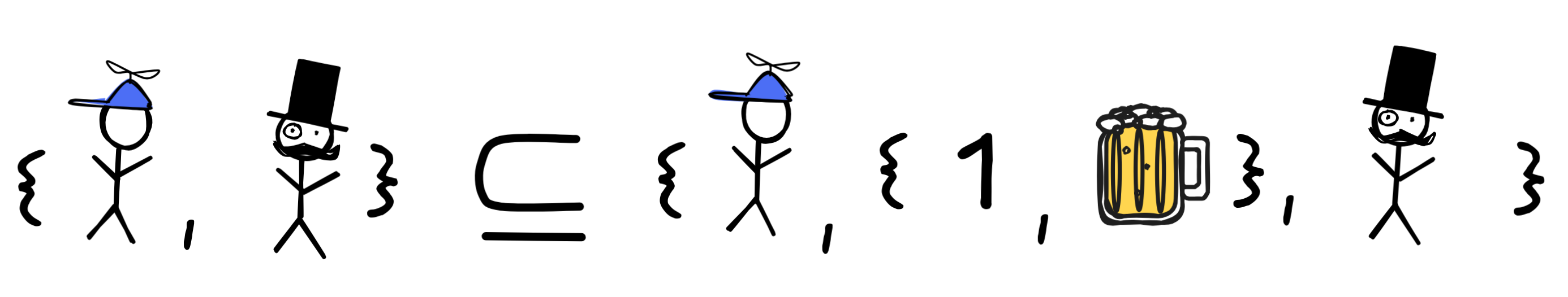
Then the latter set is a subset of the former, since both elements of the latter set—little Jimmy and Mr. Sir—are also members of the latter set:
The set that contains Mr. Sir and my beer, in contrast, is not a subset:
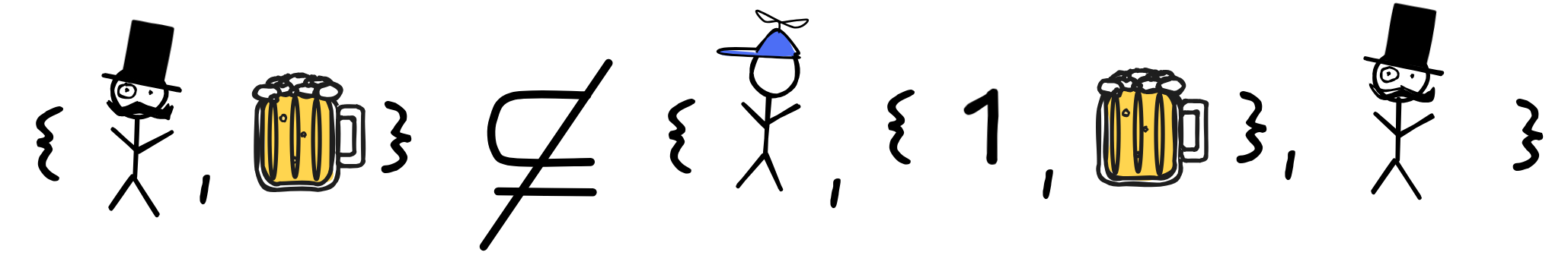
This is because the set contains my beer, which is not a member of the bigger set:
Graphically, the subset-relation amounts to one set being “enclosed by” another:
In the case of a simple inference (in a formal language), with just one premise P and conclusion C , we can directly understand deductive validity in terms of the subset relation.
The idea is that we can understand truth-preservation—the idea that the conclusion is true under the hypothesis that the premises are true—can be spelled out using models:
Single-premise deductive validity
=
In every model, where the premise P is true, the
conclusion C must be true as well.
But in set-theoretic terms that just means that the set of models of the premise
is a subset of the set of models of the conclusion:
 .
.
That is, for the inference from P to C to be valid, the situation needs to be like the one depicted here:
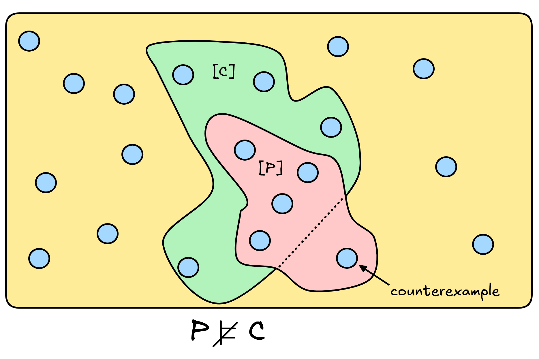
If, instead, there is a model where P is true but C is not, if there is a countermodel as depicted here, the inference is deductively invalid:
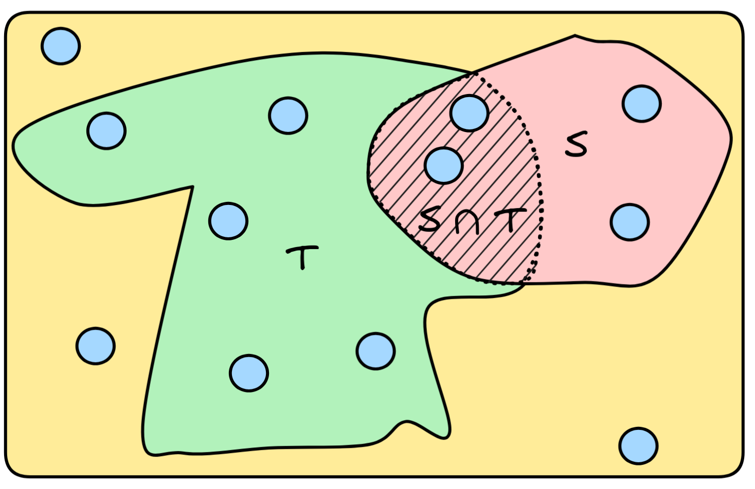
To generalize this idea to arguments with multiple premises, we need one final set-theoretic concept. The intersection of two sets S and T , denoted S ∩ T is the set that contains all and only the elements that are in both sets, i.e.
S ∩ T = { a : a ∈ S and a ∈ T}
Visually, the idea of intersection can be represented as in the following diagram, where the intersection of S and T is indicated by the shaded area:
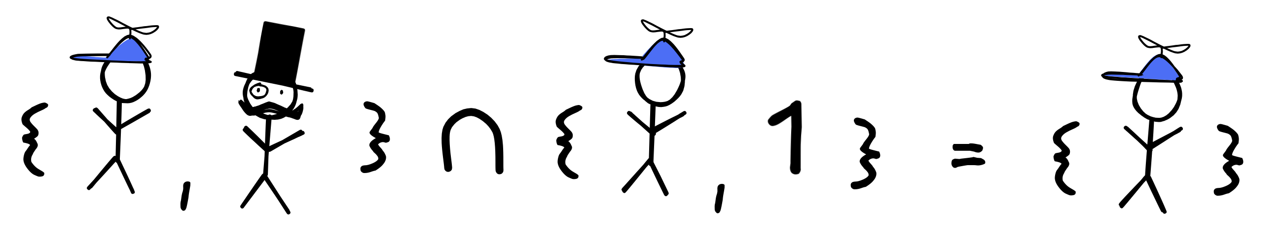
So, for example, the intersection of the set containing little Jimmy and Mr. Sir and the set containing little Jimmy and the number one is the set containing just little Jimmy:
When we have an inference with multiple premises P₁ , P₂ , …, and conclusion C , we want to say that this inference is deductively valid just in case whenever all the premises are true, so is the conclusion. That is:
General deductive validity
=
In every model, where P₁, P₂, … are all true, the
C must be true as well.
But we can describe the models where P₁ , P₂ , … are true in terms of the sets [P₁] , [P₂] , …, where each individual formula is true:
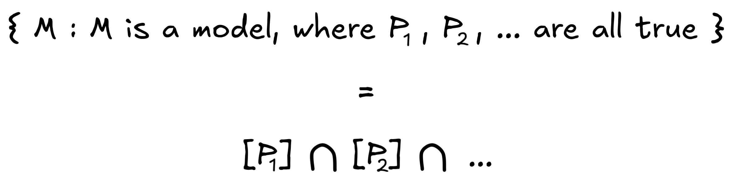
This gives us the final definition deductively valid inference:

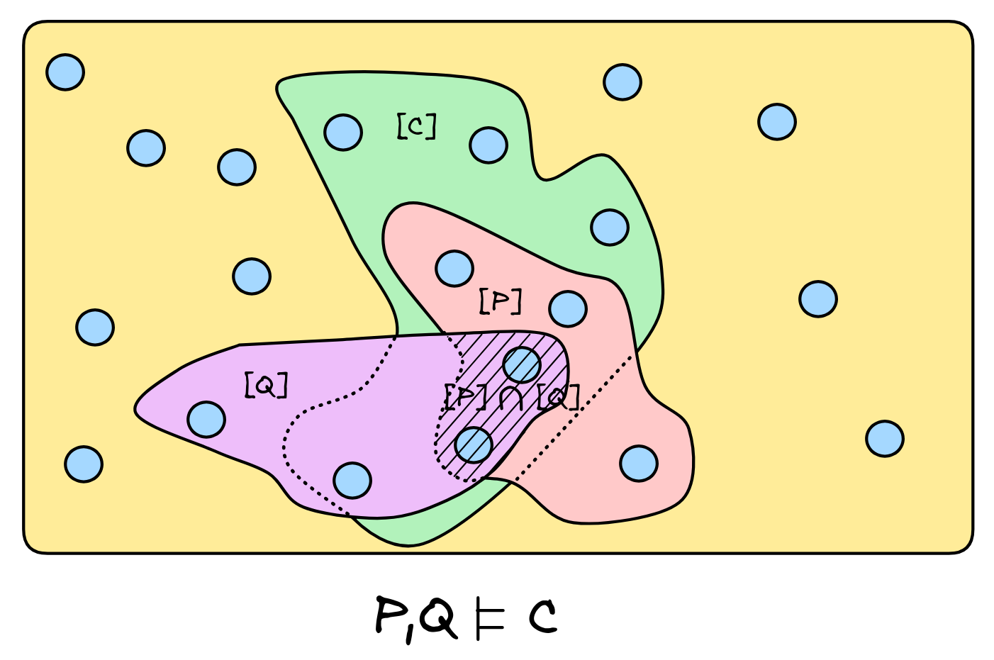
So, for an inference with two premises P,Q and conclusion C to be valid, the situation needs to like the one depicted here:
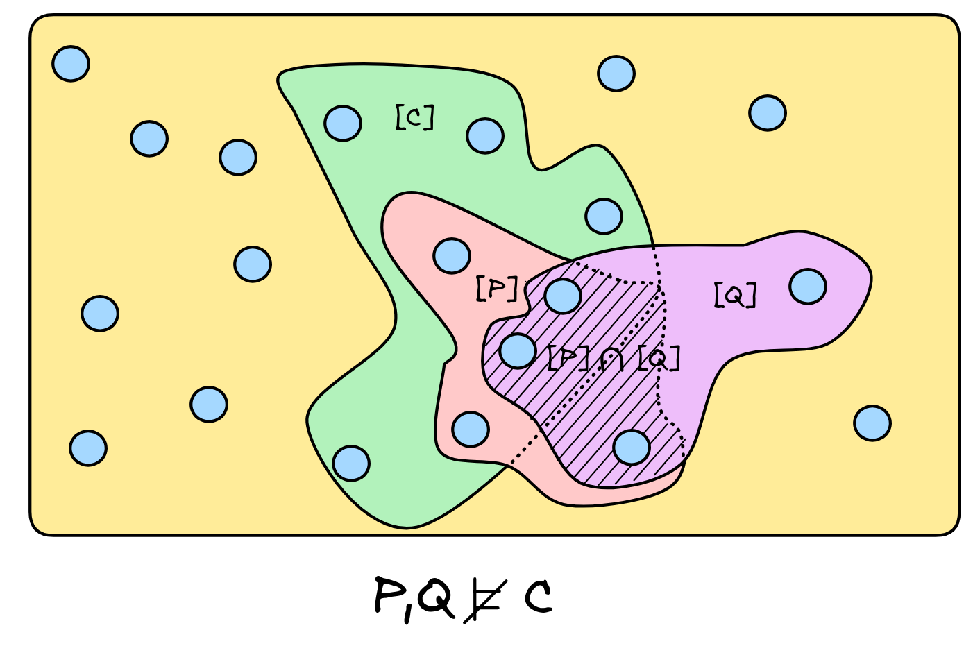
An example of a set-up, where the inference from P,Q to C is invalid is depicted here:
This is, in abstract terms, the standard logical theory of deductive inference. But it is truly abstract: we haven’t defined yet what a model really is. To obtain a workable definition for a concrete language—like the language of propositional logic—we need to supply the notion of a model for that language. What we have is a sort of blueprint for deductive validity: for any language, if we supply a definition of a model for that language and say what it means for a formula to be true in such a model, we obtain the notion of deductively valid inference in that language.
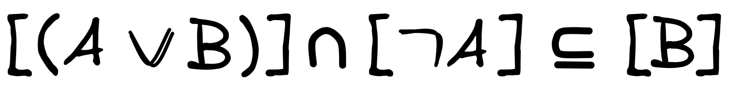
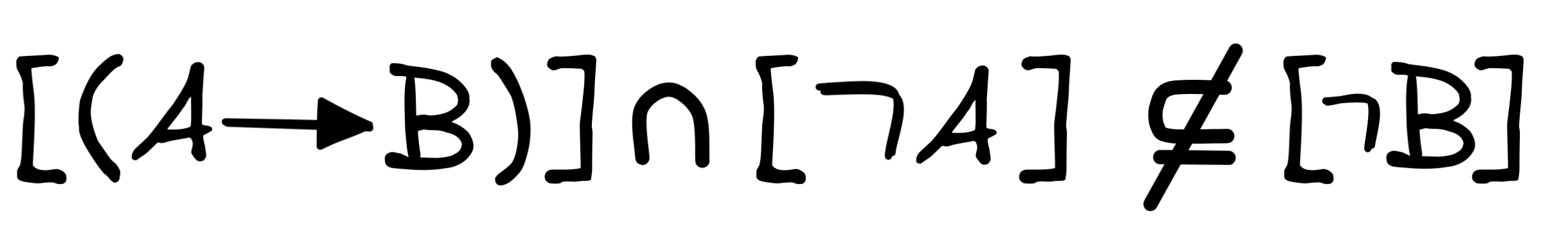
So, if we want to show that disjunctive syllogism is deductively valid in propositional logic, for example, we need to show that:
That is, we need to show that in all models where
 and
and
 are both true, B is true as well.
Similarly, if we want to show that denying the antecedent is
That is we need to show that there’s a model where
 and
are true, but
and
are true, but
 is not.
To be able to do this, we need the notion of a model for the language of propositional logic and conditions when negations, disjunctions, conditionals, and so on are true in them—providing this is the core task of semantic theory.
The concept of deductive validity is specialized. It makes sense to use deductive reasoning for specific tasks: reasoning in mathematics or other specific theories, reasoning with precisely defined concepts or pattern that are truly general. Notice how this air-tight reasoning is not quite the same thing as what Sherlock Holmes calls “doing a deduction”:
“From a drop of water… a logician could infer the possibility of an Atlantic or a Niagara without having seen or heard of one or the other. So all life is a great chain, the nature of which is known whenever we are shown a single link of it. Like all other arts, the Science of Deduction and Analysis is one which can only be acquired by long and patient study…"
Sherlock uses the word “deduction” for any reasoning that is careful, systematic, and reliable. However, the examples in this passage sounds a lot like inductive reasoning. Take a small sample and make an educated guess about the larger collection that it belongs to. That kind of reasoning is not indefeasible, it does not make a necessary connection. We do not call that deduction.
Mostly
With inductively valid inference, truth-preservation mostly holds. We’ve defined an inductively valid inference as one where if the premises are true, the conclusion is probably true. The likelihood could be slightly increased (weak induction) or greatly increased (strong induction). Either way, assuming that the premises are true gives us some reason to believe the conclusion is true. Inductive inference is not air-tight. There is a chance of going from truth to falsity, but that is a risk we have to take when we are dealing with uncertain information.
 The study of induction also has roots in ancient philosophy and psychology. The
Buddhist scholars, and brothers,
Asaṅga and
Vasubandhu focused on
inferences like “where there is smoke, there is fire”. They considered
associative thinking, tracking regularities in experience, and drawing
structural analogies to be the cornerstones of real human belief-forming
practices. This was an attempt to describe how the mind really functions to help
us navigate a world where evidence is imperfect.
The study of induction also has roots in ancient philosophy and psychology. The
Buddhist scholars, and brothers,
Asaṅga and
Vasubandhu focused on
inferences like “where there is smoke, there is fire”. They considered
associative thinking, tracking regularities in experience, and drawing
structural analogies to be the cornerstones of real human belief-forming
practices. This was an attempt to describe how the mind really functions to help
us navigate a world where evidence is imperfect.
Inductive reasoning is characteristic of scientific inference, especially in disciplines where statistical empirical research plays an important role. For example, we commonly use randomized control trials in medical research to determine the whether a drug is effective. Very roughly, the idea is that we randomly allocate participants a drug or placebo (or the like) and see if one group (drug or placebo) has significantly better outcomes. Along the way, we control for various confounding factors. If the group with the drug has better outcome than the other, we conclude that the drug is effective. This is, ultimately, a form of inductive inference: we infer that a drug works from the fact that it has worked in many cases, which have been well-sampled.—The complete story is, of course, much more complicated (how do we guarantee that we sample well, what does “significantly better” mean, …), but at the heart of this lies inductive inference.
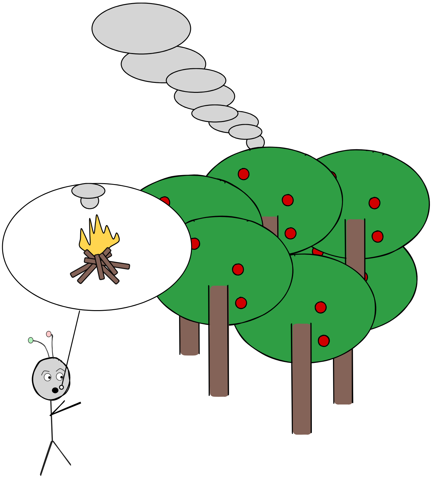
 Since inductive reasoning is defeasible—it can be
overturned by further evidence—it is well-suited to belief modulation: to
change our beliefs in light of new evidence. Take the case of smoke means fire,
for example. If IA
sees smoke coming up behind the trees, it might
think that there’s an illegal open camp-fire burning in the woods. But if IA
learns that that Mr. Sir often smokes his pipe in the forest, he might
change his conclusions. Even though the original evidence didn’t go away, it’s
been further supplemented by additional information, which changes the
conclusions we draw. In this way, inductive logic is closely related to
learning from evidence, which is a core concept of AI research.
Since inductive reasoning is defeasible—it can be
overturned by further evidence—it is well-suited to belief modulation: to
change our beliefs in light of new evidence. Take the case of smoke means fire,
for example. If IA
sees smoke coming up behind the trees, it might
think that there’s an illegal open camp-fire burning in the woods. But if IA
learns that that Mr. Sir often smokes his pipe in the forest, he might
change his conclusions. Even though the original evidence didn’t go away, it’s
been further supplemented by additional information, which changes the
conclusions we draw. In this way, inductive logic is closely related to
learning from evidence, which is a core concept of AI research.
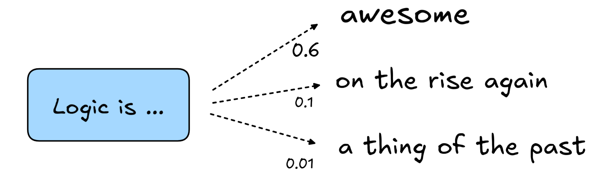
Similarly, inductive reasoning play a central role in prediction. We make predictions when we don’t know what’s going to happen: the weather, what the stock market will look like tomorrow, and so on. In fact, we’ve already discussed how next-word-prediction is essentially the core concept underlying recent AI LLMs
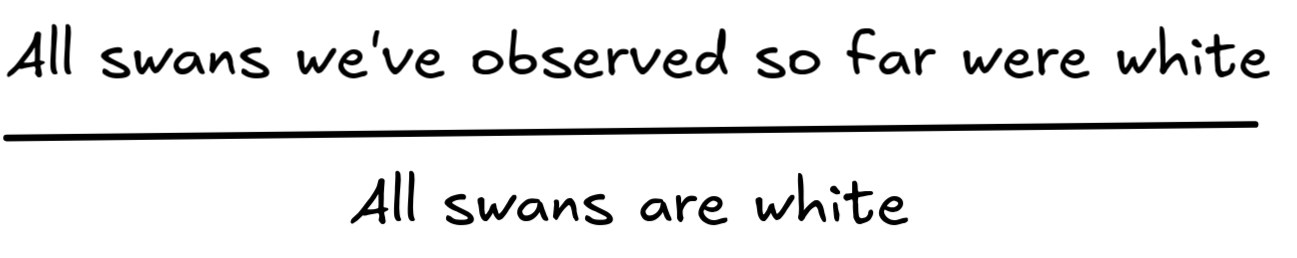
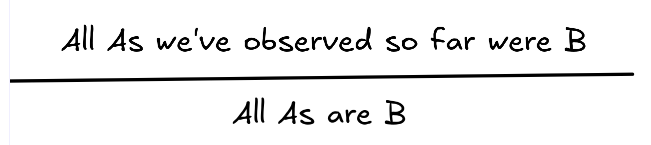
The examples we used to motivate the idea of logical form where all deductive inferences. But also inductive logic, deals with logic form. Let’s revisit some examples. First, take the inference about swans, perhaps the most traditional example of an inductive inference:
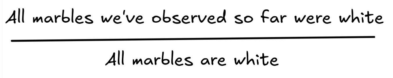
In light of the well-known fact that there are black swan’s we’ve slightly modified the example to a case where IA draws marbles from a jar:
Note that there’s the same kind of pattern going on that we’ve observed in the case of the inference about Socrates’ mortality: we can replace one predicate with another and get what looks like another inductively valid inference.
The underlying pattern of this inference is known as enumerative induction:
There are different ways in which enumerative induction is represented. Here’s another:
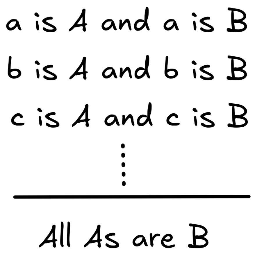
The assumption here is, of course, that a , b , c , … run through a sufficiently large number of instances.
Just like in deductive logic, we can use formal languages to mathematically represent inductive inferences. Unfortunately, however, to express inference schemas like enumerative induction, we need more expressive languages than propositional logic, so this will have to wait. But what we can talk about now, is how inductive validity is defined in formal languages in general, just like we did for deductive validity.
In inductive logic, we use the symbol
 to stand for
an inductively valid inference, writing
to stand for
an inductively valid inference, writing
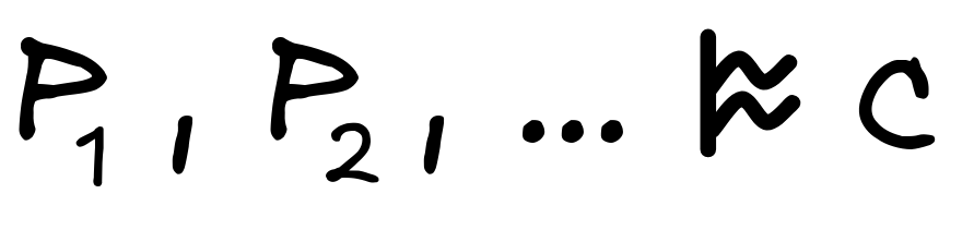 to say that the inference from the premises
P₁
,
P₂
, …,
to the conclusion
C
inductively valid. To say that an inference is inductively strong, we write a
!
on top, like so
to say that the inference from the premises
P₁
,
P₂
, …,
to the conclusion
C
inductively valid. To say that an inference is inductively strong, we write a
!
on top, like so
 . So if we have a inductively
strong inference going from premises
P₁
,
P₂
, …,
to conclusion
C
we can
abbreviate this with symbols:
. So if we have a inductively
strong inference going from premises
P₁
,
P₂
, …,
to conclusion
C
we can
abbreviate this with symbols:

There are different approaches to obtain a semantic definition of inductive validity, but the most prominent approach involves probability theory, which we use to spell out the idea of the premises making the conclusion more likely.
A straight-forward way for implementing probabilities for the formal languages of logic “piggy-backs” on the notion of a model, which we’ve used in deductive logic to define validity. So, we’ll be working with a logical space, in which each formula A has an associated set [A] of models where it is true.
In inductive logic, we think of these models as ways the world could turn out to be. If we roll a 6-sided die, for example, there are six ways the world could turn out to be: it can come up 1, 2, 3, 4, 5, or 6. Each of these corresponds to a model:
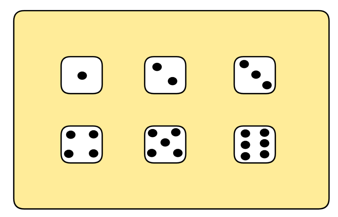
If in our language we have a formulas EVEN and ODD, for example, to say that the outcome will be even or odd, then these would correspond to the following propositions:
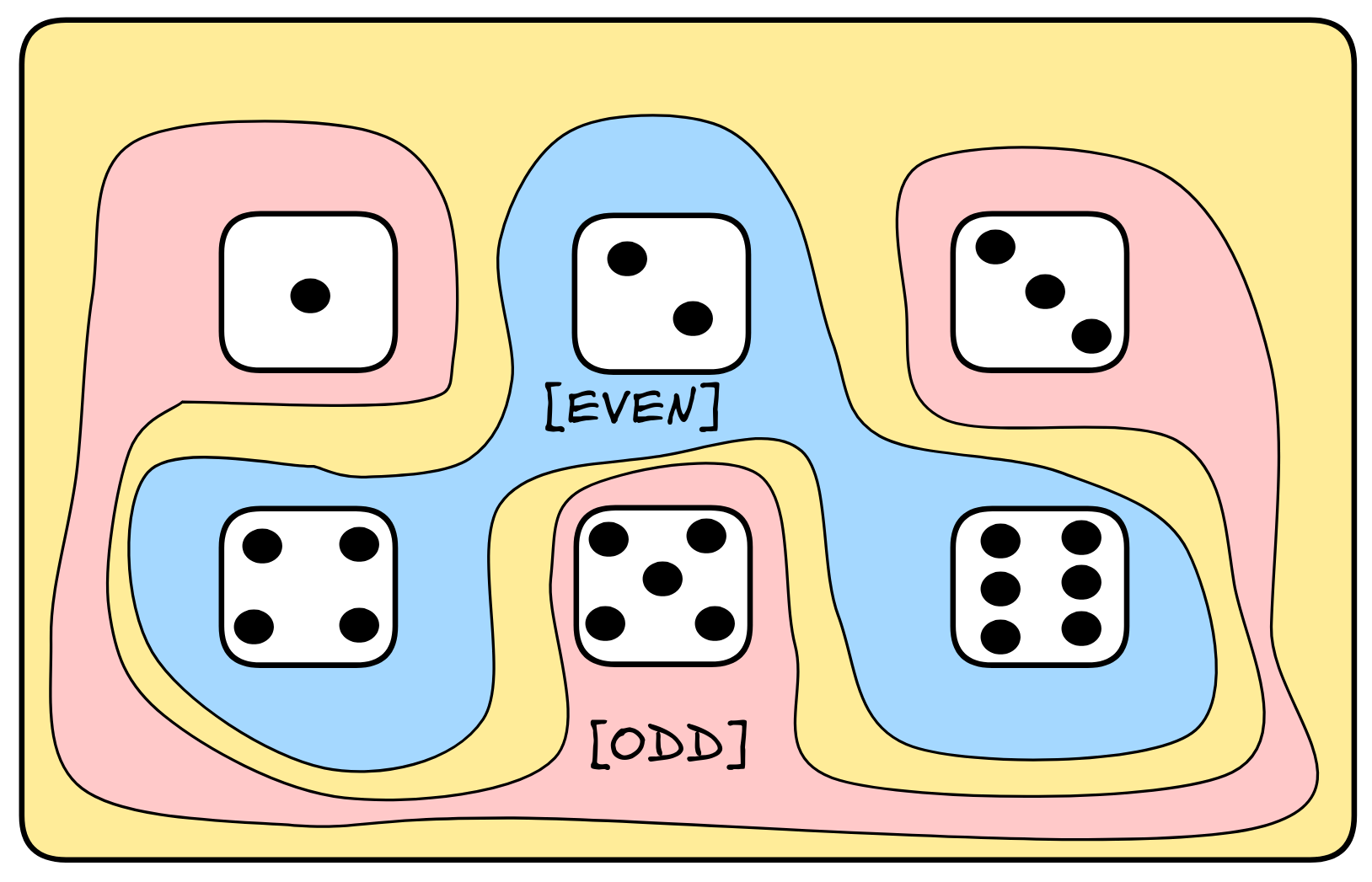
In standard probability theory, such a logical space is also known as an sample space, whose members represent different possible outcomes. In logical theory, however, the outcomes are just models: possible reasoning scenarios. The sets of models which we associate with our formulas, the propositions, are called events in standard probability theory. From the perspective of logical theory, however, they are just the semantic content of formulas.
A probability function is a mathematical function, which assigns to each propositions a real number between 0 and 1—the proposition’s probability. Well talk about the laws of probabilities when we discuss concrete systems of inductive logic, but we can outline the basic ideas of inductive logic without worrying too much about the details.
In our toy example of a die role, here’s one way the probabilities could work out:
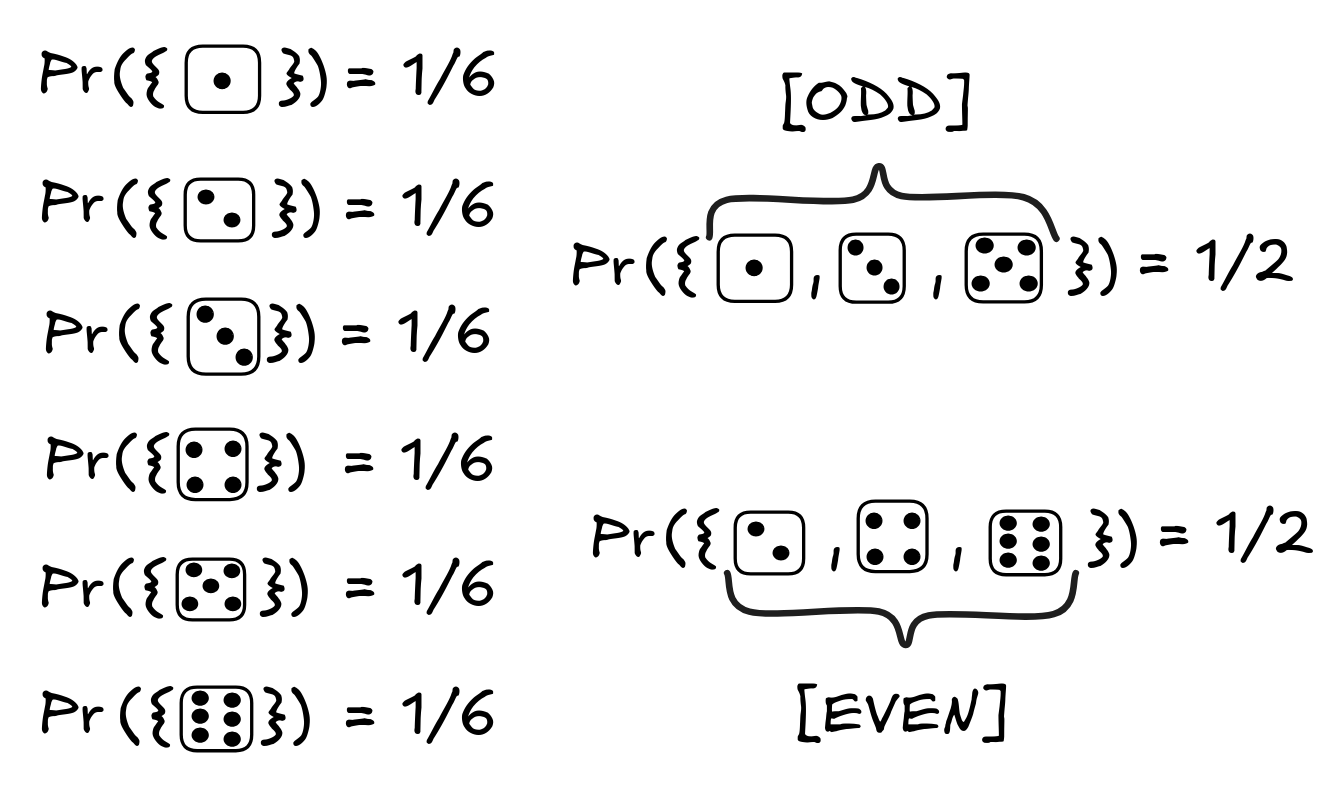
This probability distribution corresponds to the assumption that our die is fair.
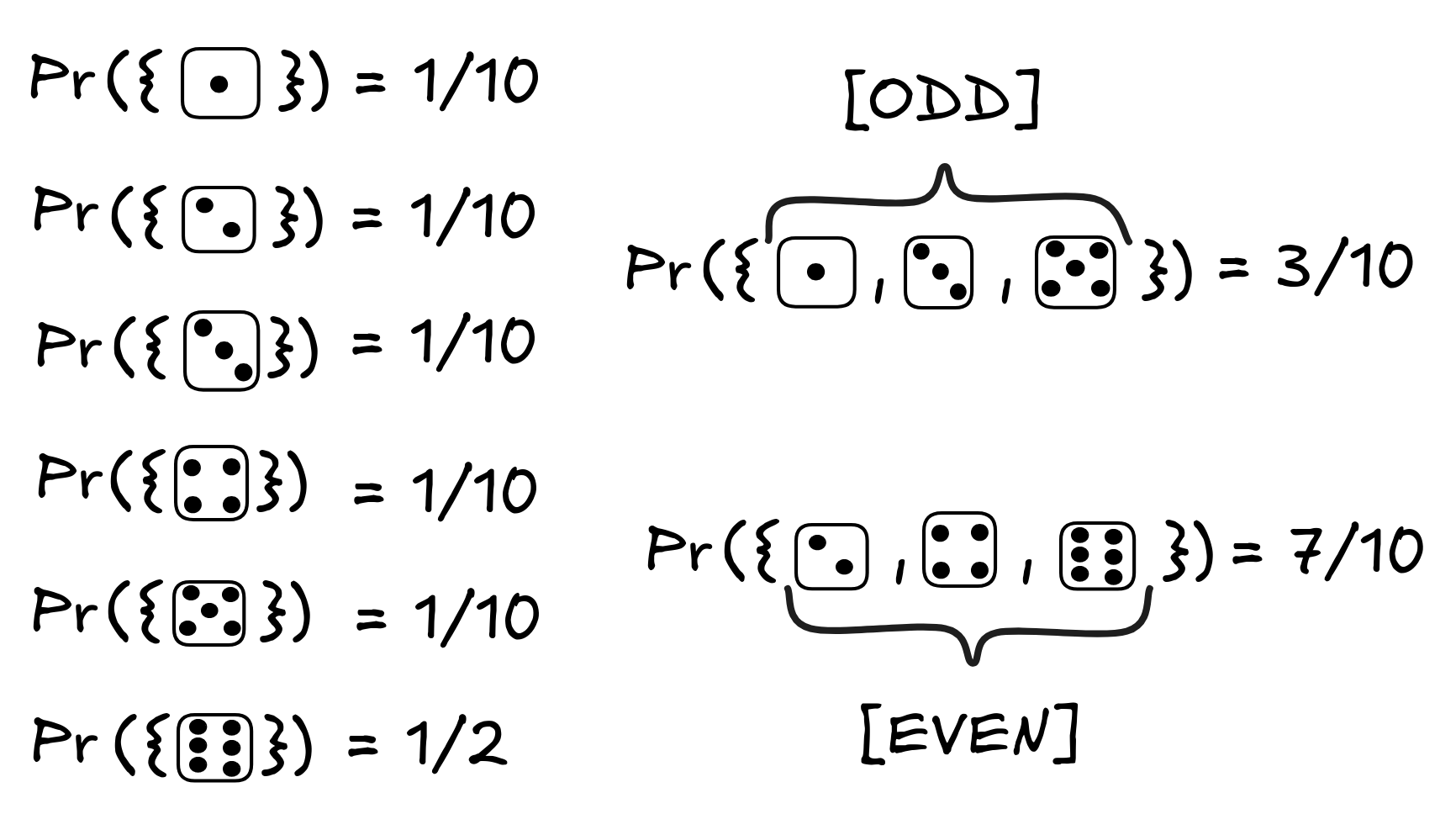
But this is not the only way the probabilities could work out. For example, if we assume that the die we’re dealing with is loaded, for example to be much more likely to roll a six, the probabilities could look like this:
We can use probabilities to mathematically spell out the idea that a conclusion is likely true on the hypothesis that the premises are. For this, we use the concept of conditional probabilities.
We write Pr([A] | [B]) to denote the conditional probability of A being true under the hypothesis that B is true. The standard definition of this is given by the following formula:
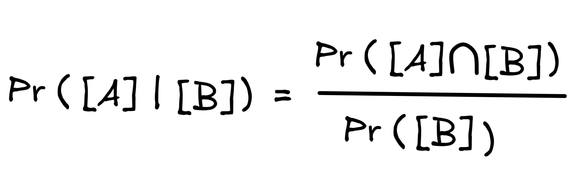
Here, we crucially need to assume that Pr([B]) ≠ 0 to avoid division by zero. What this formula says is that the conditional probability Pr([A] | [B]) of A given B is the “part” of B’s probability that is an A-probability—a measaure of the proportion of A scenarios that are B scenarios.
Here’s how this plays out in our previous two distributions if we ask ourselves what’s the probability of the role being a two given that/under the hypothesis that it’s even:
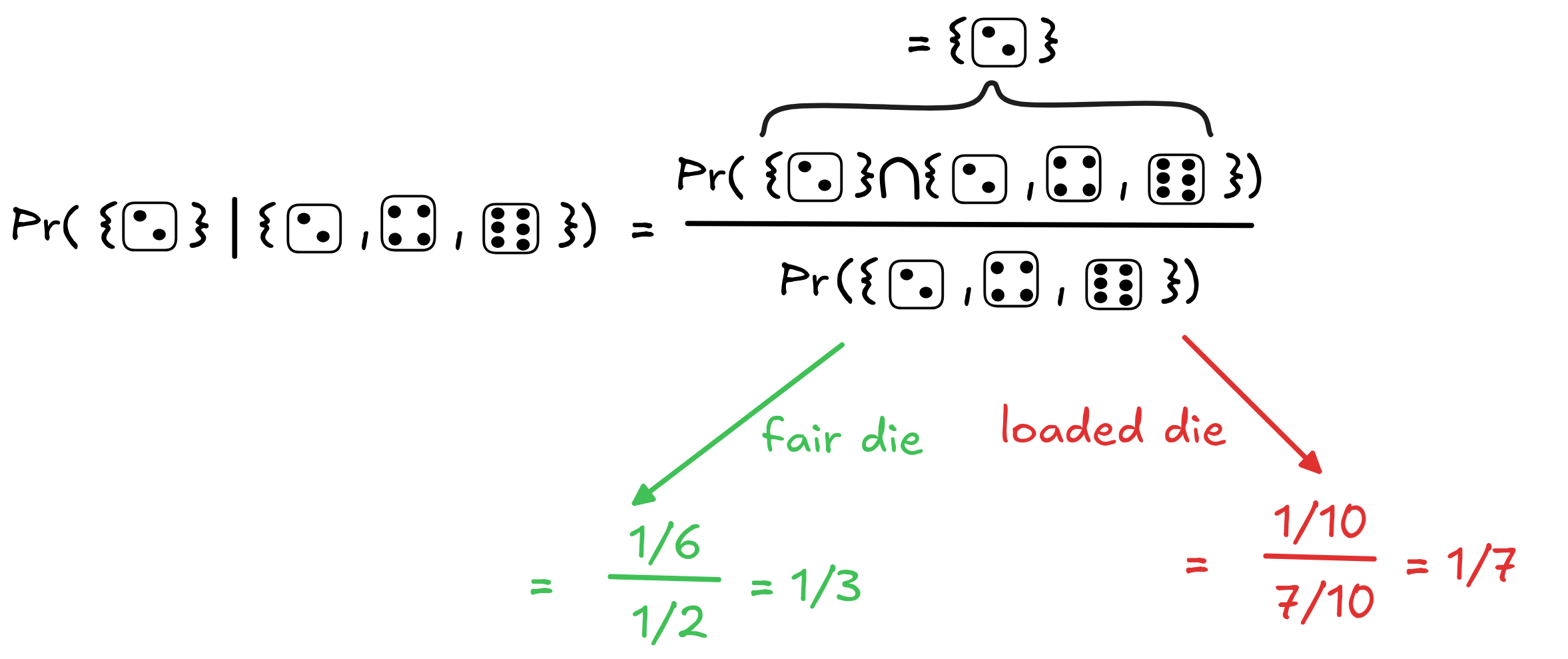
What we can see here is that the probability of the roll being a two goes up under the hypothesis that it’s even: from 1/3 to 1/2 in the case of the fair die, and from 1/10 to 1/7 in the case of the loaded die. In this sense, the hypothesis that the roll is even supports the conclusion.
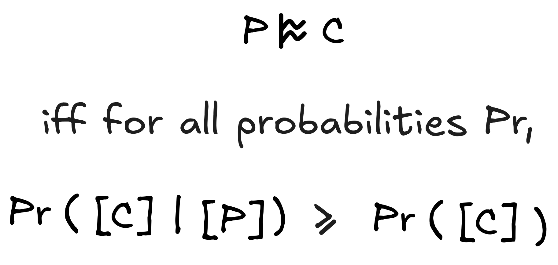
You might be worried about this increase of probabilities depending on the concrete numbers, but in fact, it doesn’t. Once we’ve introduced the laws of probability theory, we’ll be able to show that for any assignments of mathematically coherent probabilities the hypothesis that the roll is even will raise the probability of the roll being a two. This gives us a clear sense of inductively valid inference:
The strength of the inference can be determined in different ways, but the most straight-forward one is to look at the absolute increase of probability. That is, we measure the strength of an inductive inference by:
By the way: here the notation | number | stands for the absolute value of number , where, for example, | -2 | = | 2 | = 2.
In general, the strength of an inductive inference is going to depend on concrete probabilities. For example, the strength of the inference from even to two assuming a fair die is:
Instead assuming the loaded die it’s
Since 1/6 > 3/70, the inference is (much) stronger assuming a fair die (which makes sense, given that assuming a loaded die, a six becomes much more likely given that the outcome is even, while assuming a fair die, all even results go up “to the same degree”).
This gives us the chance to briefly revisit the distinction between domain-specific and domain-general, between material and logical validity. When the concrete probabilities matter in inductive inference, what we’re dealing with is material inductive inference. This kind of inference figures much more in scientific inference. Logically valid inductive inference is a much rarer phenomenon, but it underpins the basic principles of belief revision, prediction, and more.
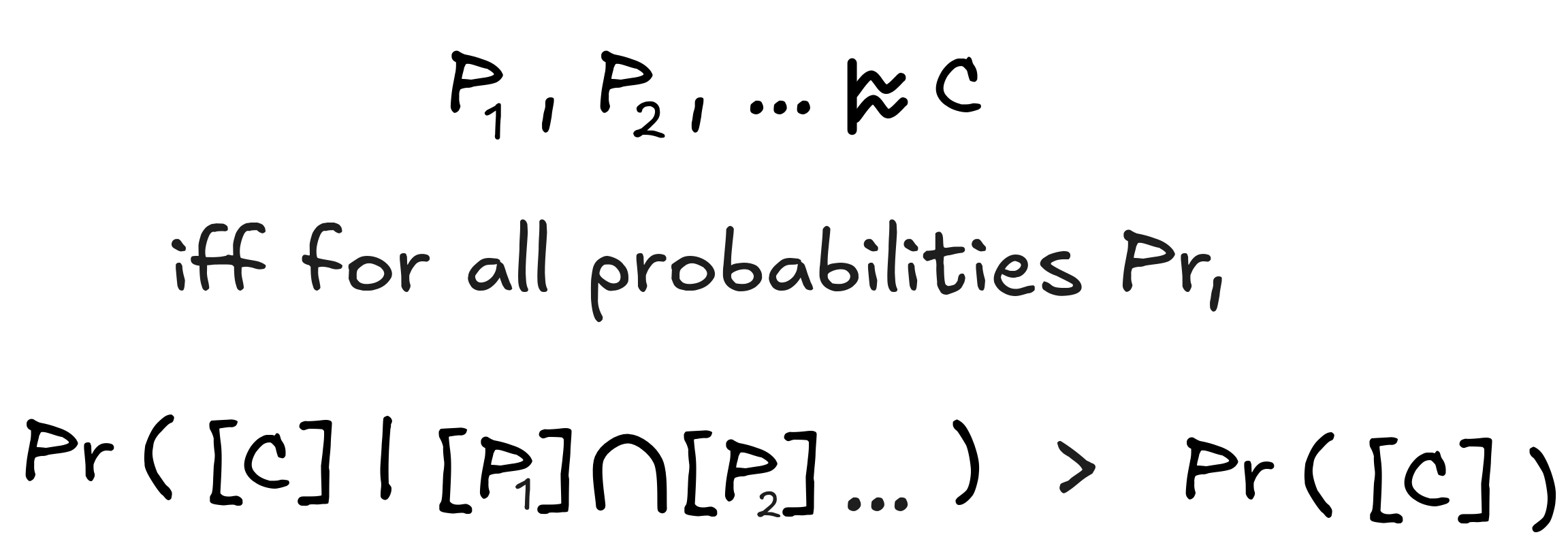
It remains to generalize the notion of inductively valid inference to inferences with more than one premise P₁ , P₂ , …, and conclusion C . But given what we know now about intersection from the study of deductive inference, this is pretty straight-forward. The obvious definition is:
Similarly, one straight-forward way of calculating the strength of the inference is:
strength = | Pr([C] | [P₁] ∩ [P₂] ∩ …) - Pr([C]) |
This gives us a blueprint for the study of inductively valid inference: once we’ve supplied a theory of models (which we’ll obtain from the study of deductive inference), all we need to supply is a theory of probabilities and we obtain a notion of inductively valid inference.
Further readings
A modern classic on the mathematical definition of deductive validity:
Update of the Tarskian method, presented at an introductory level:
Early work on AI implementations of inductive reasoning:
The idea of using probability theory to model inductive validity is heavily influenced by the work of Rudolf Carnap:
Influential mathematical treatment of inductive validity:
Last edited: 12/09/2025